Chapter 7
Localizing Errors in Data Records
7.1 Error Localization
Data can be invalidated with validation rules. If data is marked as invalid, what are the subsequent actions one should take? One possible action is to remove all invalid observations from the data. Although this may seem a sound advice, often this has severe consequences: removing all observations that contain invalid values may lead to the following:
- remove many valid and useful values,
- leave too little data to be analyzed,
- introduce selection bias in the resulting data.
Removing observations with invalid data may result in a dataset that is not representative. In many cases, the erroneous records are very relevant for the research question at hand. In statistical practice, such observations often describe difficult-to-measure subpopulations that differ from the rest of the the population and are of interest for policy makers or from a scientific point of view. Examples of interesting populations in social statistics where survey data often suffer from incomplete and erroneous observations are elderly, migrants, foreign workers, students, and homeless people. Examples in economic data are startups, flex workers, and customer-to-customer sales. Removing such records can heavily bias the statistical estimates that follow. As an extreme example, suppose that every case contains a single invalid or missing value. Removing each invalid case would then result in no data at all, thereby wasting all the observed values that are valid.
An alternative for removing invalid data is to “correct” the invalid data through data editing so that the edited data can be used in the data analysis. Changing (scientific) data for further analysis may seem wrong but often is the lesser of the two evils: having no or heavily biased data versus minimally edited data. Moreover, in some cases, the measurement error causing violation of the validation rules can be reconstructed or properly estimated. In this sense, the whole editing process can be viewed as part of the estimation procedure (van der Loo et al., 2017).
The overall data-editing strategy we follow is to detect invalid data, determine which values are considered faulty, and remove those values so that they can be imputed in later steps. This procedure thus generates missing values, and they should be chosen so that these can be imputed in a way so that no rule violations remain. As a guiding principle, we therefore demand that the original data is altered as little as possible while ensuring that the data is no longer invalidated by validation rules.
The ability to correct values requires that data errors can be identified. The procedure to find errors is referred to as error localization: which values of the data are causing invalidation and are therefore considered to be errors?
An error localization procedure must thus search the space of field combinations to find those combinations of fields that can be altered to satisfy a set of validation rules. The space of possibilities is large, and in principle, the solution need not be unique. Most error localization procedures are restricted to classes of rules that can be evaluated for each case (record) separately. That is, to check whether a case contains valid data, one only needs access to the data in that particular record. No reference to other records or datasets is necessary. Since there are less fields to consider, this restriction on the ruleset makes the problem of error localization more manageable. Moreover, error localization procedures are aimed at minimizing the (weighted) number of fields to adapt, to stay as close to the original data as possible. To clarify this, let us have a look at some examples.
For univariate rules, error localization is trivial: if an observation is invalidated by an univariate validation rule, the value of the corresponding variable is invalid.
Univariate rules are variable domain definitions: they define what values are allowed. For numeric variables, univariate rules are defined as one or more ranges, and for categorical variables they are defined as the set of allowed discrete values.
Error localization in a multivariate validation rule is more complex: in principle, any combination of values can be invalid.
This example illustrates that solutions to error localization problems are in general not unique. We can make the data satisfy the validation rule by changing the value of either Age or Married (or both). It is sometimes possible to leverage extra information. For example, if a person's date of birth is known from another reliable source, then this can be used to point out the field that most likely contains the error.
Things become more complicated still when multiple rules are involved that pertain to an overlapping set of variables. In that case, changing a value to satisfy one rule may cause the violation of another.
This example shows that an error localization procedure has to take all validation rules into account, including the rules that are not violated.
These examples motivate the following definition of the error localization procedure in terms of an optimization problem.
This minimization problem is named after (Fellegi and Holt, 1976), who first formulated and solved the problem for the case of categorical data under logical restrictions. Assigning a weight to each variable allows domain experts to influence which variables are more likely to be part of a solution. Since variables with a higher assigned weight are less likely to end up in the optimal solution, the weights are often referred to as ‘reliability weights’. Domain experts can assign higher reliability weights to variables they deem to have higher quality.
Over time, several algorithms have been developed for solving the error localization problem. An extensive overview of the theory is given in de Waal et al. (2011, Chapters 3–5). On one hand, there are specialized approaches that explicitly manipulate the rule set such as the branch-and-bound algorithm of de Waal and Quere (2003) and the original method of Fellegi and Holt (1976). On the other hand, there are approaches that translate the problem to a well-known general optimization problem (mixed-integer programming (MIP)). Some specialized approaches that focus on a single data type and a single type of rules exist as well.
In this chapter, we focus on the MIP approach. The advantage of a MIP approach is that it allows one to leverage existing, proven implementations of MIP solvers, either commercial or open source. The main downside of the MIP approach compared to the branch-and-bound algorithm is that users have less fine-grained influence on the chosen solution. Indeed, MIP solvers often return just one of the optimal solutions when multiple equivalent solutions exist, while implementations of the branch-and-bound method often return all solutions.
In the rest of this chapter, we first describe the usage of the errorlocate package. This section is then followed by a description of the translation of the error localization problem into a MIP-problem for the linear, categorical, and conditional validation rules. We end the chapter with describing the numerical stability of the implemented algorithm and give suggestions on handling potential issues.
7.2 Error Localization with R
7.2.1 The Errorlocate Package
The errorlocate package offers a small set of functions that allows users to localize errors in records that are to be validated by a set of linear, categorical, or conditional validation rules using a fast implementation of the Fellegi–Holt paradigm. Erroneous values can be automatically replaced with NA or another chosen value. The package is extensible by allowing users to implement their own error location routines. The package integrates with the validate package, which is used for rule definition and manipulation.
In errorlocate, three types of rules can be treated. First, linear rules express linear (in)equality conditions on numerical variables. Examples include (account) balance equations or nonnegativity restrictions. Second, categorical rules express conditional relations (logical implications) between two or more categorical variables. They are expressed in if-then syntax, for example, if ( age < 16) marital_status == "unmarried". Third, there are rules of mixed type. These are logical conditions where each clause consists of either a linear restriction or a restriction on categorical values. The following example illustrates how such rules can be defined in the validate package.
  rules <- validator(
    employees >= 0,                             # numerical
    profit == turnover - cost,                  # numerical
    sector   %in% c("nonprofit", "industry"),   # categorical
    bankrupt %in% c(TRUE, FALSE),               # categorical
    if (bankrupt == TRUE) sector == "industry", # categorical
    if ( sector    == "nonprofit"
       | bankrupt  == TRUE
       ) profit    <= 0,     # conditional
    if (turnover > 0) employees>= 1            # conditional
  )
The variables used in the rules are taken from the observation to be checked. It is also possible to supply one or more reference datasets that can be used in the error localization. The variables of these reference datasets are then excluded from the error localization procedure.
A Simple Example
Finding error locations with errorlocate is done with the locate_errors function. This function needs at least two parameters: a data.frame and a validator object.
The function locate_errors returns an errorlocation object that contains not only the location of errors but also some metadata and data on the process of finding the error. The location of the errors can be retrieved using the values method of errorlocation.
  library(errorlocate)
  rules <- validator(
    age >= 0
  )
  raw_data <- data.frame(age = -1, married = TRUE)
  le <- locate_errors(raw_data, rules)
  values(le)
  ##       age married
  ## [1,] TRUE   FALSE
In the example, the variable age is erroneous, since an age cannot be negative. Let us expand the example a little bit:
  library(errorlocate)
  rules <- validator(
    age >= 0,
    if (age <= 16) married == FALSE
  )
  raw_data <- data.frame(age = -1, married = TRUE)
  le <- locate_errors(raw_data, rules)
  values(le)
  ##       age married
  ## [1,] TRUE   FALSE
We have added a conditional restriction describing that a person cannot be married at the age of 16 years or younger. error_locate correctly identifies age to be a value that is causing the invalidation of both rules.
We can automatically remove errors using the replace_errors function.
  replace_errors(raw_data, rules)
  ##   age married
  ## 1  NA    TRUE
replace_errors internally calls the error_locate function. Any extra argument supplied to replace_errors will be passed through to error_locate.
What happens if age is 4?
  library(errorlocate)
  v <- validator(
    age >= 0,
    if (married==TRUE) age >= 16
  )
  raw_data <- data.frame( age     = 4
                        , married = TRUE)
  le <- locate_errors(raw_data, v)
  values(le)
  ##        age married
  ## [1,] FALSE    TRUE
Note that both age and married can be wrong. error_locate decides at random which of the variables is considered to be wrong. This is sensible since error_locate has no further information whether age or married is to be preferred. However, it is possible to supply a weight vector, matrix, or data.frame to error_locate to indicate in which value error_locate should put more trust.
  raw_data <- data.frame(age = 4, married = TRUE)
  weight <- c(age = 2, married = 1) # assuming we have a
  registration of marriages
  le <- locate_errors(raw_data, v, weight=weight)
  values(le)
  ##        age married
  ## [1,] FALSE    TRUE
Some Words on the Implementation of errorlocate
The implementation of the Fellegi–Holt algorithm is located in an R class FHErrorLocator, which is derived from the base class ErrorLocator. Each ErrorLocator object has to implement two methods.
The editrules package, the predecessor of errorlocate, implemented error localization with the branch-and-bound algorithm described by de Waal (2003) and a MIP formulation.
The main disadvantage of the branch-and-bound algorithm is that it has ![]() worst-case time and memory complexity, where
worst-case time and memory complexity, where ![]() is the number of variables occurring in a connected set of rules. Moreover, the branch-and-bound solver was written in pure R, making it intrinsically slower than a compiled language implementation. The main advantages of this approach were the ease of implementation and the opportunity for users to exert fine-grained control over the algorithm.
is the number of variables occurring in a connected set of rules. Moreover, the branch-and-bound solver was written in pure R, making it intrinsically slower than a compiled language implementation. The main advantages of this approach were the ease of implementation and the opportunity for users to exert fine-grained control over the algorithm.
7.3 Error Localization as MIP-Problem
The error localization problem can be translated to a MIP-problem. This allows us to reuse well-established results from the field of linear and MIP. Indeed, many advanced algorithms for solving such problems have been developed, and in many cases, implementations in a compiled language are available under a permissive license. In errorlocate, the solver of the lp_solve library (Berkelaar et al., 2010) is used through R's lpSolveAPI package (Konis, 2011). The lp_solve library is written in ANSI C and has been tried and tested extensively.
The strategy to solve error localization problems through this library from R therefore consists of translating the problem to a suitable MIP-problem, feeding this problem to lpSolveAPI, and translating the results back to an error location. It is necessary to distinguish among the following:
- linear restrictions on purely numerical data,
- restrictions on purely categorical data, and
- conditional restrictions on mixed-type data,
since restriction for each data type calls for a different translation to a MIP problem.
We will focus on how to translate these types of error localization problems to a mixed-integer formulation, paying attention to both theoretical and practical details. In Section 7.4, attention is paid to numerical stability issues and Section 7.2 is devoted to examples in R code.
7.3.1 Error Localization and Mixed-Integer Programming
A MIP-problem is an optimization problem that can be written in the form

where ![]() is a constant vector and
is a constant vector and ![]() is a vector consisting of real and integer coefficients. One usually refers to
is a vector consisting of real and integer coefficients. One usually refers to ![]() as the decision vector and the inner product
as the decision vector and the inner product ![]() as the objective function. Furthermore,
as the objective function. Furthermore, ![]() is a coefficient matrix and
is a coefficient matrix and ![]() a vector of upper bounds. Formally, the elements of
a vector of upper bounds. Formally, the elements of ![]() ,
, ![]() , and
, and ![]() are limited to the rational numbers (Schrijver, 1998). This is never a problem in practice since we are always working with a computer representation of numbers.
are limited to the rational numbers (Schrijver, 1998). This is never a problem in practice since we are always working with a computer representation of numbers.
The name MIP stems from the fact that ![]() contains continuous as well as integer variables. When
contains continuous as well as integer variables. When ![]() consists solely of continuous or integer variables, Problem (7.1) reduces, respectively, to a linear or an integer programming problem. An important special case occurs when the integer coefficients of
consists solely of continuous or integer variables, Problem (7.1) reduces, respectively, to a linear or an integer programming problem. An important special case occurs when the integer coefficients of ![]() may only take values from {0,1}. Such variables are often called binary variables. It occurs as a special case since defining
may only take values from {0,1}. Such variables are often called binary variables. It occurs as a special case since defining ![]() to be integer and applying the appropriate upper bounds yield the same problem.
to be integer and applying the appropriate upper bounds yield the same problem.
MIP is well understood, and several software packages are available that implement efficient solvers. Most MIP software support a broader, but equivalent, formulation of the MIP problem, allowing the set of restrictions to include inequalities as well as equalities. As a side note we mention that under equality restrictions, solutions for the integer part of ![]() are only guaranteed to exist when the equality restrictions pertaining to the integer part of
are only guaranteed to exist when the equality restrictions pertaining to the integer part of ![]() are totally unimodular.1 However, as we will see below, restrictions on
are totally unimodular.1 However, as we will see below, restrictions on ![]() are always inequalities in our case, so this is of no particular concern to us.
are always inequalities in our case, so this is of no particular concern to us.
We reformulate Fellegi–Holt error localization (Fellegi and Holt, 1976) for numerical, categorical, and mixed-type restrictions in terms of MIP problems. The precise reformulations of the error localization problem for the three types of rules are different, but in each case the objective function is of the form
where ![]() is a vector of positive weights and
is a vector of positive weights and ![]() a vector of binary variables, one for each variable in the original record, that indicates whether its value should be replaced. More precisely, for a record
a vector of binary variables, one for each variable in the original record, that indicates whether its value should be replaced. More precisely, for a record ![]() of
of ![]() variables, we define
variables, we define

This objective function obviously meets the requirement that the minimal (weighted) number of variables should be replaced. In general, a record may contain numeric, categorical, or both types of data, and restrictions may pertain to either one or both data types. To distinguish between the data types below, we shall write ![]() , where
, where ![]() represents the categorical and
represents the categorical and ![]() the numerical part of
the numerical part of ![]() .
.
For an error localization problem, the restrictions of Problem (7.1) consist of two parts, which we denote

Here, the restrictions indicated with ![]() represent a matrix representation of the user-defined (hard) restrictions that the original record
represent a matrix representation of the user-defined (hard) restrictions that the original record ![]() must obey. The vector
must obey. The vector ![]() contains at least a numerical representation of the values in a record
contains at least a numerical representation of the values in a record ![]() and the binary variables
and the binary variables ![]() . An algorithmic MIP solver will iteratively alter the values of
. An algorithmic MIP solver will iteratively alter the values of ![]() until a solution satisfying (7.4) is reached. To make sure that the objective function reflects the (weighted) number of variables altered in the process, the restrictions in
until a solution satisfying (7.4) is reached. To make sure that the objective function reflects the (weighted) number of variables altered in the process, the restrictions in ![]() serve to make sure that the values in
serve to make sure that the values in ![]() that represent values in
that represent values in ![]() cannot be altered without setting the corresponding value in
cannot be altered without setting the corresponding value in ![]() to 1.
to 1.
Summarizing, in order to translate the error localization problem for the special cases of linear, categorical, or conditional mixed-type restrictions to a general MIP-problem, for each case we need to properly define ![]() , the restriction set
, the restriction set ![]() , and the restriction set
, and the restriction set ![]() .
.
7.3.2 Linear Restrictions
For a numerical record ![]() taking values in
taking values in ![]() , a set of linear restrictions can be written as
, a set of linear restrictions can be written as
where in errorlocate, we allow the set of restrictions to contain equalities, inequalities (![]() ), and strict inequalities (
), and strict inequalities (![]() ). The formulation of these rules is very close to the formulation of the original MIP problem of Eq. (7.1). The vector to minimize over is defined as follows:
). The formulation of these rules is very close to the formulation of the original MIP problem of Eq. (7.1). The vector to minimize over is defined as follows:
with the ![]() as in Eq. (7.3). The set of restrictions
as in Eq. (7.3). The set of restrictions ![]() is equal to the set of restrictions of Eq. (7.5), except in the case of strict inequalities. The reason is that while
is equal to the set of restrictions of Eq. (7.5), except in the case of strict inequalities. The reason is that while errorlocate allows the user to define strict inequalities (![]() ), the
), the lpsolve library used by errorlocate only allows for inclusive inequalities (![]() ). For this reason, strict inequalities of the form
). For this reason, strict inequalities of the form ![]() are rewritten as
are rewritten as ![]() , with
, with ![]() a suitably small positive constant.
a suitably small positive constant.
In the case of linear rules, the set of constraints ![]() consists of pairs of the form
consists of pairs of the form

for ![]() . Here,
. Here, ![]() are the actual observed values in the record and
are the actual observed values in the record and ![]() a suitably large positive constant allowing
a suitably large positive constant allowing ![]() to vary between
to vary between ![]() and
and ![]() . It is not difficult to see that if
. It is not difficult to see that if ![]() is different from
is different from ![]() , then
, then ![]() must equal 1. For, if we choose
must equal 1. For, if we choose ![]() , we obtain the set of restrictions
, we obtain the set of restrictions
which states that ![]() equals
equals ![]() .
.
7.3.3 Categorical Restrictions
Categorical records ![]() take values in a Cartesian product domain
take values in a Cartesian product domain
where each ![]() is a finite set of categories for the
is a finite set of categories for the ![]() categorical variable. The category names are unimportant, so we write
categorical variable. The category names are unimportant, so we write
The total number of possible value combinations ![]() is equal to the product of the
is equal to the product of the ![]() .
.
A categorical edit is a subset ![]() of
of ![]() where records are considered invalid, and we may write
where records are considered invalid, and we may write
where each ![]() is a subset of
is a subset of ![]() . It is understood that if a record
. It is understood that if a record ![]() , then the record violates the edit. Hence, categorical rules are negatively formulated (they specify the region of
, then the record violates the edit. Hence, categorical rules are negatively formulated (they specify the region of ![]() where
where ![]() may not be) in contrast to linear rules that are positively formulated (they specify the region of
may not be) in contrast to linear rules that are positively formulated (they specify the region of ![]() where
where ![]() must be). To be able to translate categorical rules to a MIP problem, we need to specify
must be). To be able to translate categorical rules to a MIP problem, we need to specify ![]() such that if
such that if ![]() , then
, then ![]() satisfies
satisfies ![]() . Here,
. Here, ![]() is the complement of
is the complement of ![]() in
in ![]() , which can be written as
, which can be written as
where for each variable ![]() ,
, ![]() is the complement of
is the complement of ![]() in
in ![]() . Observe that Eq. (7.12) states that if at least one
. Observe that Eq. (7.12) states that if at least one ![]() , then
, then ![]() satisfies
satisfies ![]() . Below, we will use this property and construct a linear relation that counts the number of
. Below, we will use this property and construct a linear relation that counts the number of ![]() over all variables.
over all variables.
To be able to formulate the Fellegi-Holt problem in terms of a MIP problem, we first associate with each categorical variable ![]() a binary vector
a binary vector ![]() of which the coefficients are defined as follows (see also Eq. (7.9)):
of which the coefficients are defined as follows (see also Eq. (7.9)):

where ![]() . Thus, each element of
. Thus, each element of ![]() corresponds to one category in
corresponds to one category in ![]() . It is zero everywhere except at the value of
. It is zero everywhere except at the value of ![]() . We will write
. We will write ![]() to indicate the concatenated vector
to indicate the concatenated vector ![]() , which represents a complete record. Similarly, each edit can be represented by a binary vector
, which represents a complete record. Similarly, each edit can be represented by a binary vector ![]() given by
given by

where we interpret 1 and 0 as TRUE and FALSE, respectively, and the logical 'or' (![]() ) is applied element-wise to the coefficients of
) is applied element-wise to the coefficients of ![]() . The above relation can be interpreted as stating that
. The above relation can be interpreted as stating that ![]() represents the valid value combinations of variables contained in the edit.
represents the valid value combinations of variables contained in the edit.
To set up the hard restriction matrix ![]() of Eq. (7.4), we first impose the obvious restriction that each variable can take but a single value:
of Eq. (7.4), we first impose the obvious restriction that each variable can take but a single value:

for ![]() . It is now not difficult to see that the demand (Eq. (7.12)) that at least one of the
. It is now not difficult to see that the demand (Eq. (7.12)) that at least one of the ![]() may be written as
may be written as
Eqs. (7.15) and (7.16) constitute the hard restrictions, stored in ![]() .
.
Using the binary vector notation for ![]() , and adding the
, and adding the ![]() variables that indicate variable change, the vector to minimize over (Eq. (7.1)) is written as
variables that indicate variable change, the vector to minimize over (Eq. (7.1)) is written as
To ensure that a change in ![]() results in a change in
results in a change in ![]() , the matrix
, the matrix ![]() contains the restrictions
contains the restrictions
for ![]() . Here,
. Here, ![]() is the observed value for variable
is the observed value for variable ![]() . One may check, using Eq. (7.13), that the above equation can only hold when either
. One may check, using Eq. (7.13), that the above equation can only hold when either ![]() and
and ![]() (the original value is retained) or
(the original value is retained) or ![]() and
and ![]() (the value changes).
(the value changes).
7.3.4 Mixed-Type Restrictions
Records ![]() containing both numerical and categorical data can be denoted as a concatenation of categorical and numerical variables taking values in
containing both numerical and categorical data can be denoted as a concatenation of categorical and numerical variables taking values in ![]() :
:
where ![]() is defined in Eq. (7.9). As stated earlier, categorical edits are usually defined negatively as a region of
is defined in Eq. (7.9). As stated earlier, categorical edits are usually defined negatively as a region of ![]() that is disallowed, while linear rules define regions in
that is disallowed, while linear rules define regions in ![]() that are allowed. We may choose a negative formulation of rules containing both variable types by defining a single rule
that are allowed. We may choose a negative formulation of rules containing both variable types by defining a single rule ![]() as follows:
as follows:
where ![]() and
and ![]() is a convex subset of
is a convex subset of ![]() defined by a (possibly empty) set of
defined by a (possibly empty) set of ![]() linear inequalities of the form
linear inequalities of the form ![]() . It is understood that if
. It is understood that if ![]() , then
, then ![]() violates the rule. An example of a restriction pertaining to a categorical and a numerical variable is ‘A company employs staff if and only if it has positive personnel cost’. The corresponding rule can be denoted as
violates the rule. An example of a restriction pertaining to a categorical and a numerical variable is ‘A company employs staff if and only if it has positive personnel cost’. The corresponding rule can be denoted as ![]() .
.
To obtain a positive reformulation, we first negate the set membership condition and apply basic rules of proposition logic:
This then yields a positive formulation of ![]() . That is, a record
. That is, a record ![]() satisfies
satisfies ![]() if and only if
if and only if

Observe that this formulation allows one to define multiple disconnected regions in ![]() containing valid records using just a single rule. For example, one may define a numeric variable to be either smaller than 0 or larger than 1. This type of restriction cannot be formulated using just linear numerical restrictions.
containing valid records using just a single rule. For example, one may define a numeric variable to be either smaller than 0 or larger than 1. This type of restriction cannot be formulated using just linear numerical restrictions.
This formulation is both a generalization of linear inequality (Eq. (7.5)) and categorical rules (Eq. (7.11)). Choosing ![]() , we get
, we get ![]() , and only the categorical part remains. Similarly, choosing
, and only the categorical part remains. Similarly, choosing ![]() , only the disjunction of linear inequalities remains. A system of linear equations that must simultaneously be obeyed like in Eq. (7.5) can be obtained by defining multiple rules
, only the disjunction of linear inequalities remains. A system of linear equations that must simultaneously be obeyed like in Eq. (7.5) can be obtained by defining multiple rules ![]() , each containing a single linear restriction.
, each containing a single linear restriction.
The definition in Eq. (7.22) can be rewritten as a ‘conditional rule’ using the implication replacement rule from propositional logic, which states that ![]() may be replaced by
may be replaced by ![]() . If we limit Eq. (7.22) to a single inequality, we obtain the normal form of de Waal (2003).
. If we limit Eq. (7.22) to a single inequality, we obtain the normal form of de Waal (2003).
If we choose ![]() and leave two inequalities, we obtain a conditional rule on numerical data:
and leave two inequalities, we obtain a conditional rule on numerical data:
Writing mixed-type rules in conditional form seems more user-friendly as they can directly be translated into an if statement in a scripting language. Finally, note that equalities can be introduced by defining pairs of rules like the following:

To reformulate Eq. (7.22) as a MIP problem, we first define binary variables ![]() that indicate whether
that indicate whether ![]() obeys
obeys ![]() :
:

Using the or-form of the set condition (Eq. (7.22)), we can write the mixed-data rule as
Recall from Eqs. (7.14) and (7.13) that ![]() is the binary vector representation of a categorical rule and
is the binary vector representation of a categorical rule and ![]() the binary vector representation of a categorical record. In the above equation, the ‘
the binary vector representation of a categorical record. In the above equation, the ‘![]() ’ is the arithmetic translation of the logical ‘
’ is the arithmetic translation of the logical ‘![]() ’ operator in Eq. (7.22) that connects the categorical with the linear restrictions. When any one of the two terms is positive, record
’ operator in Eq. (7.22) that connects the categorical with the linear restrictions. When any one of the two terms is positive, record ![]() satisfies rule
satisfies rule ![]() .
.
Rules of this form constitute the user-defined part of the ![]() part of the restriction matrix. To explicitly identify
part of the restriction matrix. To explicitly identify ![]() with the linear restrictions, we also add
with the linear restrictions, we also add
to ![]() with
with ![]() a suitably large positive constant. Indeed, if
a suitably large positive constant. Indeed, if ![]() , the inequality
, the inequality ![]() is enforced, and Eq. (7.28) always is satisfied. When
is enforced, and Eq. (7.28) always is satisfied. When ![]() , the whole restriction can hold regardless of whether the inequality holds. Finally, similar to the purely categorical case, we need to add restrictions on the binary representation of
, the whole restriction can hold regardless of whether the inequality holds. Finally, similar to the purely categorical case, we need to add restrictions on the binary representation of ![]() as in Eq. (7.15), so Eqs. (7.15) (7.28), and (7.29) constitute
as in Eq. (7.15), so Eqs. (7.15) (7.28), and (7.29) constitute ![]() .
.
There may be multiple mixed-type rules, each yielding one or more ![]() indicator variables for each rule. The decision vector for the MIP problem may therefore be written as
indicator variables for each rule. The decision vector for the MIP problem may therefore be written as
where ![]() is the total number of linear rules occurring in all the mixed-type rules. Finally, the
is the total number of linear rules occurring in all the mixed-type rules. Finally, the ![]() matrix connecting the change indicator variables (
matrix connecting the change indicator variables (![]() ) with the actual recorded values consists of the union of the restrictions for categorical variables (Eq. (7.18)) and those for numerical variables (Eq. (7.7)).
) with the actual recorded values consists of the union of the restrictions for categorical variables (Eq. (7.18)) and those for numerical variables (Eq. (7.7)).
7.4 Numerical Stability Issues
An error localization problem, in its original formulation, is an optimization problem over ![]() binary decision variables that indicate which variables in a record should be adapted. Depending on the type of rules, its reformulation as a MIP problem adds at least
binary decision variables that indicate which variables in a record should be adapted. Depending on the type of rules, its reformulation as a MIP problem adds at least ![]() variables and
variables and ![]() restrictions. Moreover, the reformulation as a MIP problem introduces a constant
restrictions. Moreover, the reformulation as a MIP problem introduces a constant ![]() , the value of which has no mathematical significance but for which a value must be chosen in practice. Because of limitations in machine accuracy, which is typically on the order of
, the value of which has no mathematical significance but for which a value must be chosen in practice. Because of limitations in machine accuracy, which is typically on the order of ![]() , the range of problems that can be solved is limited as well. In particular, MIP problems that involve both very large and very small numbers in the objective function and/or the restriction matrix may yield erroneous solutions or become numerically unfeasible. Indeed, the manual of
, the range of problems that can be solved is limited as well. In particular, MIP problems that involve both very large and very small numbers in the objective function and/or the restriction matrix may yield erroneous solutions or become numerically unfeasible. Indeed, the manual of lp_solve (Berkelaar et al., 2010) points out that ‘[…] to improve stability, one must try to work with numbers that are somewhat in the same range. Ideally, in the neighborhood of 1’. The following sections point out a number of sources of numerical instabilities and provide ways to handle them.
7.4.1 A Short Overview of MIP Solving
Consider a set of linear restrictions on numerical data of the form ![]() , where we assume
, where we assume ![]() , and the restrictions consist solely of inequalities (
, and the restrictions consist solely of inequalities (![]() ). In practice, these restrictions will not limit the type of linear rules covered by this discussion, since it can be shown that all linear rules can be brought to this form, possibly by introducing dummy variables [see, e.g., Bradley et al. (1977); Schrijver (1998)]. Furthermore, suppose that we have a record
). In practice, these restrictions will not limit the type of linear rules covered by this discussion, since it can be shown that all linear rules can be brought to this form, possibly by introducing dummy variables [see, e.g., Bradley et al. (1977); Schrijver (1998)]. Furthermore, suppose that we have a record ![]() that does not obey the restrictions. The MIP formulation of the error localization problem can be written as follows:
that does not obey the restrictions. The MIP formulation of the error localization problem can be written as follows:

and ![]() . Also,
. Also, ![]() denotes the unit matrix,
denotes the unit matrix, ![]() a vector with all coefficients equal to 1, and
a vector with all coefficients equal to 1, and ![]() . The last row is added to force
. The last row is added to force ![]() . This is necessary because we will initially treat the binary variables
. This is necessary because we will initially treat the binary variables ![]() as if they are real numbers in the range
as if they are real numbers in the range ![]() .
.
The lp_solve library uses an approach based on the revised Phase I– Phase II simplex algorithm to solve MIP problems. In this approach, every inequality of Eq. (7.31) is transformed to an equality by adding dummy variables: each row ![]() is replaced by
is replaced by ![]() , with
, with ![]() . Depending on the sign of the inequality, the extra variable
. Depending on the sign of the inequality, the extra variable ![]() is called a slack or surplus variable. In Eq. (7.31), there are four sets of restrictions (rows). We therefore need to add four sets of surplus and slack variables (columns) in order to rewrite the whole system in terms of equalities.
is called a slack or surplus variable. In Eq. (7.31), there are four sets of restrictions (rows). We therefore need to add four sets of surplus and slack variables (columns) in order to rewrite the whole system in terms of equalities.
Note that after this transformation, the whole problem including the cost function is written in terms of equalities. It is customary to organize this set of equality objective function in a single tableau notation as follows:
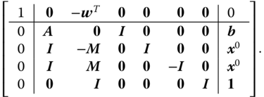
Here, the first row and column represent the cost function. Columns 2 and 3 correspond to the original set of variables in Eq. (7.31), while columns 4-7 correspond to sets of slack and surplus variables. The final column contains the constant vector.
A tableau representation shows all the numbers that are relevant in an LP problem at a glance. By examining how LP solvers typically manipulate these numbers, we gain some insight into how and where numerical stability issues may arise.
Since the tableau represents a set of linear equalities, it may be manipulated as such. In fact, the simplex method is based on performing a number of cleverly chosen Gauss–Jordan elimination steps on the tableau. For a complete discussion, the reader is referred to one of the many textbooks discussing it (e.g., Bradley et al. (1977)), but in short, the Phase I–Phase II simplex algorithm consists of the following steps:
- Phase I.
Repeatedly apply Gauss–Jordan elimination steps (called pivots) to derive a decision vector that obeys all restrictions. A vector obeying all restrictions is called a basic solution.
- Phase II.
Repeatedly apply pivots to move from the initial nonoptimal solution to the solution that minimizes the objective function
 .
.
In Phase I, a decision vector ![]() (with
(with ![]() the vector of slack and surplus variables) is derived that obeys all restrictions. The precise algorithm need not be described here. It involves adding again extra variables where necessary and then manipulating the system of equalities represented by the tableau so that those extra variables are driven to zero. The binary variables
the vector of slack and surplus variables) is derived that obeys all restrictions. The precise algorithm need not be described here. It involves adding again extra variables where necessary and then manipulating the system of equalities represented by the tableau so that those extra variables are driven to zero. The binary variables ![]() are first treated as if they are real variables. In Appendix 7.A, it is shown in detail how an initial solution for Eq. (7.32) can be found; here, we just state the result of a Phase I operation:
are first treated as if they are real variables. In Appendix 7.A, it is shown in detail how an initial solution for Eq. (7.32) can be found; here, we just state the result of a Phase I operation:

This tableau immediately suggests a valid solution: it is easily confirmed by matrix multiplication that the vector ![]() obeys all restrictions. In the above form of a tableau, where the restriction matrix contains (a column permutation of) the unit matrix, the right-hand side has only nonnegative coefficients, and the cost vector equals zero for the columns above the unit matrix, which is called the canonical form.
obeys all restrictions. In the above form of a tableau, where the restriction matrix contains (a column permutation of) the unit matrix, the right-hand side has only nonnegative coefficients, and the cost vector equals zero for the columns above the unit matrix, which is called the canonical form.
Now, a pivot operation consists of the following steps:
- 1. Select a positive element
 from the restriction matrix. This is called the pivot element.
 - 2. Multiply the
 th row by
  .
. - 3. Subtract the
 th row, possibly after rescaling, from all other rows of the tableau such that their
  th column equals zero.
The result of a pivot operation is again a tableau in canonical form but with possibly a different value for the cost function. The simplex algorithm proceeds by selecting pivots that decrease the cost function until the minimum is reached or the problem is shown to be unfeasible.
Up until this point, we have treated the binary variables ![]() as if they were real variables, so the tableaux discussed above do not represent solutions to our original problem, which demands that all
as if they were real variables, so the tableaux discussed above do not represent solutions to our original problem, which demands that all ![]() are either 0 or 1. In the
are either 0 or 1. In the lp_solve library, this is solved as follows:
- 1. For each optimized value
 , test whether it is 0 or 1. If all
  are integers, we have a valid solution of objective value
  , and we are done.
 - 2. For the first variable
 that is not integer, create two submodels: one where the minimum value of
  equals 1, and one where the maximum value of
  equals 0.
 - 3. Optimize the two submodels. If solutions exist, the result will contain an integer
 .
. - 4. For the submodels that have a solution and whose current objective value does not exceed that of an earlier found solution, return to step 1.
The above branch-and-bound approach completes this overview. The discussion of pivot and branch-and-bound operations has so far been purely mathematical: no choices have been made regarding issues such as how to decide when the floating-point representation of a value is regarded zero, or how to handle badly scaled problems. Do note, however, that in the course of going from Phase I to Phase II, the LP solver is handling numbers that may range from ![]() to
to ![]() , which typically differ many orders of magnitude.
, which typically differ many orders of magnitude.
7.4.2 Scaling Numerical Records
In the MIP formulation of error localization over numerical records under linear restrictions, Eq. (7.7) restricts the search space around the original value ![]() to
to ![]() . This restriction may prohibit a MIP solver from finding the actual minimal set of values to adapt or even render the MIP problem unsolvable. As an example, consider the following error localization problem on a two-variable record:
. This restriction may prohibit a MIP solver from finding the actual minimal set of values to adapt or even render the MIP problem unsolvable. As an example, consider the following error localization problem on a two-variable record:

Obviously, the record can be made to obey the restriction by multiplying ![]() by
by ![]() or by dividing
or by dividing ![]() by the same amount. However, in
by the same amount. However, in errorlocate, the default value for ![]() , which renders the corresponding MIP problem unsolvable. Practical example where such errors occur is when a value is recorded in the wrong unit of measure (e.g., in € instead of k€.).
, which renders the corresponding MIP problem unsolvable. Practical example where such errors occur is when a value is recorded in the wrong unit of measure (e.g., in € instead of k€.).
It is therefore advisable to remove such unit-of-measure errors prior to error localization2 and to express numerical records on a scale such that all ![]() . Note that under linear restrictions (Eq. (7.5)) one may always apply a scaling factor
. Note that under linear restrictions (Eq. (7.5)) one may always apply a scaling factor ![]() to a numerical record
to a numerical record ![]() by replacing
by replacing ![]() with
with ![]() . In the above example, one may replace
. In the above example, one may replace ![]() by
by ![]() for the purpose of error localization. If
for the purpose of error localization. If ![]() and the coefficients of
and the coefficients of ![]() do not vary over many orders of magnitude, such a scaling will suffice to numerically stabilize the MIP problem.
do not vary over many orders of magnitude, such a scaling will suffice to numerically stabilize the MIP problem.
7.4.3 Setting Numerical Threshold Values
On most modern computer systems, real numbers are represented in IEEE (2008) double precision format. In essence, real numbers are represented as rounded-off fractions so that arithmetic operations on such numbers always result in loss of precision and round-off errors. For example, even though mathematically we have ![]() , in the floating-point representation (denoted
, in the floating-point representation (denoted ![]() ), we have
), we have ![]() . In fact, the difference is about
. In fact, the difference is about ![]() in this case.
in this case.
This means that in practice one cannot rely on equality tests to determine whether two floating-point numbers are equal. Rather, one considers two numbers ![]() and
and ![]() equal when
equal when ![]() is smaller than a predefined tolerance. For this reason,
is smaller than a predefined tolerance. For this reason, lp_solve comes with a number of predefined tolerances. These tolerances have default values, but these may be altered by the user.
The tolerances implemented by lp_solve are summarized in Table 7.1. The value of epspivot is used to determine whether an element of the restriction matrix is positive so that it may be used as a pivoting element. Its default value is ![]() , but note that after Phase I, our restriction matrix contains elements on the order of
, but note that after Phase I, our restriction matrix contains elements on the order of ![]() . For this reason, the value of
. For this reason, the value of epspivot is lowered in errorlocate by default, but users may override these settings. For the same reason, the value of epsint, which determines when a value for one of the ![]() can be considered integer, is lowered in
can be considered integer, is lowered in errorlocate as well. The other tolerance settings of lp_solve, epsb (to test if the right-hand side of the restrictions differs from 0), epsd (to test if two values of the objective function differ), epsel (all other values), and mip_gap (to test whether a bound condition has been hit in the branch-and-bound algorithm), have not been altered.
The limited precision inherent to floating-point calculations implies that computations get more inaccurate as the operands differ more in magnitude. For example, on any system that uses double precision arithmetic, the difference ![]() is indistinguishable from
is indistinguishable from ![]() . This, then, leads to two contradictory demands on our translation of an error localization problem to a MIP problem. On one hand, one would like to set
. This, then, leads to two contradictory demands on our translation of an error localization problem to a MIP problem. On one hand, one would like to set ![]() as large as possible so that the ranges
as large as possible so that the ranges ![]() contain a valid value of
contain a valid value of ![]() . On the other hand, large values for
. On the other hand, large values for ![]() imply that MIP problems such as Eq. (7.31) may become numerically unstable.
imply that MIP problems such as Eq. (7.31) may become numerically unstable.
In practice, the tableau used by lp_solve will not be exactly the same as represented in Eq. (7.33). Over the years, many optimizations and heuristics have been developed to make solving linear programming problems fast and reliable, and several of those optimizations have been implemented in lp_solve. However, the tableau of Eq. (7.33) does fundamentally show how numerical instabilities may occur: the tableau simultaneously contains numbers on the order of ![]() and on the order of
and on the order of ![]() . It is not at all unlikely that the two differ in many orders of magnitude.
. It is not at all unlikely that the two differ in many orders of magnitude.
The above discussion suggests the following rules of thumb to avoid numerical instabilities in error localization problems:
- 1. Make sure that elements of
 are expressed in units such that
  ,
,  , and
, and  are on the order of 1 wherever possible.
 - 2. Choose a value of
 appropriate for
  .
. - 3. If the above does not help in stabilizing the problem, try lowering the numerical constants of Table 7.1.
In our experience, the settings denoted in Table 7.1 have performed well in a range of problems where elements of ![]() and
and ![]() are on the order of 1 and values of
are on the order of 1 and values of ![]() are in the range
are in the range ![]() . However, these settings have been made configurable so that users may choose their own settings as needed.
. However, these settings have been made configurable so that users may choose their own settings as needed.
Table 7.1 Numerical parameters for MIP-based error localization
| Default value | |||
| Parameter | lp_solve |
errorlocate |
Description |
M |
— | Set bounds so |
|
eps |
— | Translate |
|
epspivot |
Test pivot element |
||
epsint |
Test |
||
epsb |
Test |
||
epsd |
Test obj. values |
||
epsel |
Test other numbers |
||
mip_gap |
Test obj. values |
||
7.5 Practical Issues
The following sections provide some background that can aid in choosing a set of reliability weights or to make a error localization problem more tractable by showing how certain rules can be simplified.
7.5.1 Setting Reliability Weights
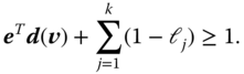
The error localization problem can be reformulated as follows: For a record ![]() violating one or more validation rules imposed on it, find the set of variables
violating one or more validation rules imposed on it, find the set of variables ![]() of which the values can be altered such that (1)
of which the values can be altered such that (1) ![]() satisfies all restrictions and (2) the sum
satisfies all restrictions and (2) the sum

is minimized. Here, the vector ![]() is a vector of chosen reliability weights. Solutions
is a vector of chosen reliability weights. Solutions ![]() that satisfy restriction (1) are called feasible solutions, and solutions that satisfy (2) are called minimal feasible solutions. We also denote with
that satisfy restriction (1) are called feasible solutions, and solutions that satisfy (2) are called minimal feasible solutions. We also denote with ![]() the size of the solution. The solution for which
the size of the solution. The solution for which ![]() is minimal is called the feasible solution of minimal size.
is minimal is called the feasible solution of minimal size.
When all weights are equal, the solution found by the error localization procedure is the solution that alters the least number of variables: in that case the solution of minimal weight is equal to the solution of minimal size. If the weights differ enough across the variables, this is not necessarily the case anymore, the solution of minimal weight may contain more variables than the solution of minimal size. As an example, suppose that there are ![]() variables. We find for a certain error localization problem that there are three feasible solutions:
variables. We find for a certain error localization problem that there are three feasible solutions: ![]() ,
, ![]() , and the trivial solution
, and the trivial solution ![]() . If the weight vector
. If the weight vector ![]() , we find that
, we find that ![]() is the solution of minimal size, while
is the solution of minimal size, while ![]() is the solution of minimal weight.
is the solution of minimal weight.
In practice, weights are often determined by domain experts, based on their experience with repeatedly analyzing a type of dataset. One question arising in this context is whether it is possible to choose a set of weights such that the solution of minimal weight can be guaranteed to be a solution of minimal size. Such a set of weights then represents the guiding principle that states that we wish to change as few values as possible while still allowing to control the localization procedure with information on the relative reliability of variables. Perhaps surprisingly, it is possible to create such a vector. To show this we will derive the following result (this is a slightly stricter version of the result in van der Loo (2015a)).
We can apply this result to construct a rescaling for any weight vector so that the feasible solution of minimal weight becomes a feasible solution of minimal size.

Here, we defined ![]() so that
so that ![]() . This of course ensures that
. This of course ensures that ![]() .
.
To illustrate this scaling, return again to the example with ![]() ,
, ![]() , and feasible solutions
, and feasible solutions ![]()
![]() and
and ![]() . After scaling, we get
. After scaling, we get ![]() , so
, so ![]() ,
, ![]() , and
, and ![]() .
.
7.5.2 Simplifying Conditional Validation Rules
Validation rules that combine linear (in)equality restrictions can put a severe performance burden on the error localization algorithm. Depending on the algorithm, the computational time needed for error localization may be as much as double with each extra conditional rule. In the case of MIP solving, a conditional rule means the introduction of dummy variables that increase the size of the problem. There are some cases, however, where conditional restrictions on combinations of linear inequalities can be simplified and rewritten into a set of pure inequalities. Here, we discuss two types of (partial) rule sets where simplification is possible.
Case 1
The first type is a ruleset of the form

As a practical example, one can think of ![]() as the number of employees and
as the number of employees and ![]() as wages paid. Both cannot be negative, and if there are any employees, some wages must have been paid. Figure 7.1(a) shows in gray the valid region corresponding to this ruleset in the
as wages paid. Both cannot be negative, and if there are any employees, some wages must have been paid. Figure 7.1(a) shows in gray the valid region corresponding to this ruleset in the ![]() -plane. The black dots correspond to valid combinations of
-plane. The black dots correspond to valid combinations of ![]() and
and ![]() , while the crosses correspond to invalid combinations. Now as depicted in 7.1(b), if we replace the conditional rule with
, while the crosses correspond to invalid combinations. Now as depicted in 7.1(b), if we replace the conditional rule with ![]() , with some appropriately chosen
, with some appropriately chosen ![]() , the valid region shrinks somewhat, while all valid observations remain valid, and all invalid observations remain invalid. So, the question is what choice of
, the valid region shrinks somewhat, while all valid observations remain valid, and all invalid observations remain invalid. So, the question is what choice of ![]() would be appropriate, given some observed pairs
would be appropriate, given some observed pairs ![]() . This is stated in the following result:
. This is stated in the following result:

Figure 7.1 (a) In gray, the area of valid combinations  according to the rule set of Eq. (7.36), black dots represent valid combinations, and crosses represent invalid combinations. The
  -axis is part of the valid area. (b) The valid area is defined by
  and
and  , with an appropriate choice for
  .
.
In the above calculation, the smallest possible value for ![]() was chosen so that the replacing rule still works. In practice, one can choose for
was chosen so that the replacing rule still works. In practice, one can choose for![]() some reasonable minimum. For example, suppose again that
some reasonable minimum. For example, suppose again that ![]() stands for number of employees and
stands for number of employees and ![]() for wages paid. The smallest nonzero value for
for wages paid. The smallest nonzero value for ![]() would then be 1, and the value
would then be 1, and the value ![]() is then the smallest wage that can be paid to an employee.
is then the smallest wage that can be paid to an employee.
Case 2
Now, consider a second type of ruleset, given by

Again, we can think of ![]() as number of employees and of
as number of employees and of ![]() as wages paid. The ruleset then states that wages are paid if and only if the number of employees is positive. Figure 7.2(a) shows in gray the associated valid region in the
as wages paid. The ruleset then states that wages are paid if and only if the number of employees is positive. Figure 7.2(a) shows in gray the associated valid region in the ![]() -plane. Black dots again depict valid observations, while crosses depict invalid observations. In Figure 7.2(b), we see the valid regions bordered by the lines
-plane. Black dots again depict valid observations, while crosses depict invalid observations. In Figure 7.2(b), we see the valid regions bordered by the lines ![]() and
and ![]() . The question is, again what values for
. The question is, again what values for ![]() and
and ![]() to choose?
to choose?
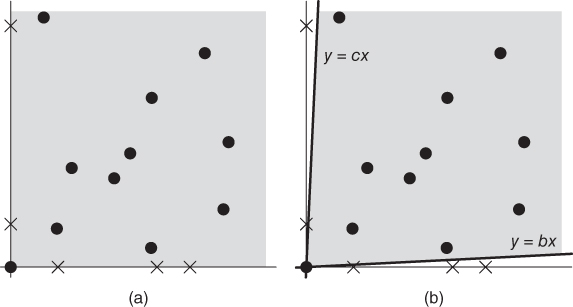
Figure 7.2 (a) In gray, the area of valid combinations  according to the rule set of Eq. (7.39). Black dots represent valid combinations, and crosses represent invalid combinations. The
  -axis is part of the valid area. (b) The valid area is defined by
  ,
,  , and
, and  with appropriate choices for
  and
and  .
.
As an example, consider a dataset on hospitals, where ![]() is the number of beds and
is the number of beds and ![]() the number of patients occupying a bed. These numbers cannot be negative. We also assume that if a hospital has beds, then there must be a patient (hospitals are never empty), and if there is at least one patient, there must be a nonzero number of beds. This amounts to the ruleset
the number of patients occupying a bed. These numbers cannot be negative. We also assume that if a hospital has beds, then there must be a patient (hospitals are never empty), and if there is at least one patient, there must be a nonzero number of beds. This amounts to the ruleset

Using the above proposition, we can replace this ruleset with the simpler

Here, ![]() is the smallest number of beds per patient, which we can choose equal to 1.
is the smallest number of beds per patient, which we can choose equal to 1. ![]() is the largest number of beds per patient or the inverse of the smallest occupancy rate that can reasonably be expected for a hospital.
is the largest number of beds per patient or the inverse of the smallest occupancy rate that can reasonably be expected for a hospital.
Generalizations
Finally, we state a few simple generalizations of the above simplifications. The proofs of these generalizations follow the same reasoning as the proofs for Propositions 7.5.10 and 7.5.11 and will not be stated here.
7.6 Conclusion
When a record is invalidated by a set of record scoped rules, it can be a problem to identify which fields are likely to be responsible for the error. In this chapter, we have seen that these fields can be indentified using the Fellegi–Holt formalism. This error localization problem for linear, categorical, and mixed-type restrictions can be formulated in terms of a MIP-problem. Mixed-type restrictions can be seen as a generalization of both record-wise linear and categorical restrictions. MIP-problems can be solved.
Although MIP-problems can be solved by readily available software packages, there may be a trade-off in numerical stability with respect to a branch-and-bound approach. This holds especially when typical default settings of such software are left unchanged and data records and/or linear coefficients of the restriction sets cover several orders of magnitude. In this paper, we locate the origin of these instabilities and provide some pointers to avoiding such problems.
The lp_solve package has now been introduced as a MIP solver back end to our errorlocate R package for error localization and rule management. Our benchmarks indicate that in generic cases where no prior knowledge is available about which values in a record may be erroneous (as may be expressed by lower reliability weights), the MIP method is much faster than the previously implemented branch-and-bound-based algorithms. On the other hand, the branch-and-bound-based approach returns extra information, most notably the number of equivalent solutions. The latter can be used as an indicator for quality of automatic data editing.
Appendix 7.A: Derivation of Eq. (7.33)
In the Phase I–Phase II simplex method, Phase I is aimed to derive a valid solution, which is then iteratively updated to an optimal solution in Phase II. Here, we derive a Phase I solution, specific for error localization problems.
Recall the tableau of Eq. (7.32); for clarity, the top row indicates to what variables the columns of the tableau pertain to.

Here, the ![]() are slack or surplus variables, aimed to write the original inequality restrictions as equalities. The
are slack or surplus variables, aimed to write the original inequality restrictions as equalities. The ![]() are used to rewrite restrictions on observed variables, the
are used to rewrite restrictions on observed variables, the ![]() to write the upper and lower limits on
to write the upper and lower limits on ![]() as equalities, and
as equalities, and ![]() to write the upper limits on
to write the upper limits on ![]() as equalities.
as equalities.
Observe that the above tableau almost suggests a trivial solution. If we choose ![]() ,
, ![]() , and
, and ![]() , we may set
, we may set ![]() . However, recall that we demand all variables to be nonnegative, so
. However, recall that we demand all variables to be nonnegative, so ![]() may not be equal to
may not be equal to ![]() . To resolve this problem, we introduce a set of artificial variables
. To resolve this problem, we introduce a set of artificial variables ![]() and extend the restrictions involving
and extend the restrictions involving ![]() as follows:
as follows:
This yields the following tableau:

The essential point to note is that the tableau now contains a unit matrix in columns 4, 5, 7, and 8, so choosing ![]() ,
, ![]() ,
, ![]() ,
, ![]() , and
, and ![]() is a solution obeying all restrictions. The artificial variables have no relation to the original problem, so we want them to be zero in the final solution. Since the tableau represents a set of linear equalities, we are allowed to multiply rows with a constant and add and subtract rows. If this is done in such a way that we are again left with a unit matrix in part of the columns, a new valid solution is generated. Here, we add the fourth row to row 3 and subtract
is a solution obeying all restrictions. The artificial variables have no relation to the original problem, so we want them to be zero in the final solution. Since the tableau represents a set of linear equalities, we are allowed to multiply rows with a constant and add and subtract rows. If this is done in such a way that we are again left with a unit matrix in part of the columns, a new valid solution is generated. Here, we add the fourth row to row 3 and subtract ![]() times the fourth row from the last row. Row 4 is multiplied with
times the fourth row from the last row. Row 4 is multiplied with ![]() . This gives
. This gives

This almost gives a new valid solution, except that the first row, representing the objective function, has not vanished at the third column. However, we may re-express the objective function in terms of the other variables, namely, using row 4, we have
Substituting this equation in the top row of the tableau shows that ![]() ,
, ![]() ,
, ![]() ,
, ![]() , and
, and ![]() represent a valid solution. Since the artificial variables have vanishing values, we may now delete the corresponding column and arrive at the tableau of Eq. (7.33).
represent a valid solution. Since the artificial variables have vanishing values, we may now delete the corresponding column and arrive at the tableau of Eq. (7.33).