
The following test objectives for Exam CX-310-202 are covered in this chapter:
Analyze and explain RAID (0, 1, 5) and SVM concepts (logical volumes, soft partitions, state databases, hot spares, and hot spare pools).
![]() A thorough understanding of the most popular RAID levels is essential to any system administrator managing disk storage. This chapter covers all the basic Solaris Volume Manager (SVM) concepts that the system administrator needs to know for the exam.
A thorough understanding of the most popular RAID levels is essential to any system administrator managing disk storage. This chapter covers all the basic Solaris Volume Manager (SVM) concepts that the system administrator needs to know for the exam.
Create the state database, build a mirror, and unmirror the root file system.
![]() The system administrator needs to be able to manipulate the state database replicas and create logical volumes, such as mirrors (RAID 1). This chapter details the procedure for creating the state databases as well as mirroring and unmirroring the root file system.
The system administrator needs to be able to manipulate the state database replicas and create logical volumes, such as mirrors (RAID 1). This chapter details the procedure for creating the state databases as well as mirroring and unmirroring the root file system.
The following strategies will help you prepare for the test:
![]() As you study this chapter, the main objective is to become comfortable with the terms and concepts that are introduced.
As you study this chapter, the main objective is to become comfortable with the terms and concepts that are introduced.
![]() For this chapter it’s important that you practice, on a Solaris system (ideally with more than one disk), each step-by-step and each command that is presented. Practice is very important on these topics, so you should practice until you can repeat each procedure from memory.
For this chapter it’s important that you practice, on a Solaris system (ideally with more than one disk), each step-by-step and each command that is presented. Practice is very important on these topics, so you should practice until you can repeat each procedure from memory.
![]() Be sure that you understand the levels of RAID discussed and the differences between them.
Be sure that you understand the levels of RAID discussed and the differences between them.
![]() Be sure that you know all of the terms listed in the “Key Terms” section at the end of this chapter. Pay special attention to metadevices and the different types that are available.
Be sure that you know all of the terms listed in the “Key Terms” section at the end of this chapter. Pay special attention to metadevices and the different types that are available.
With standard disk devices, each disk slice has its own physical and logical device. In addition, with standard Solaris file systems, a file system cannot span more than one disk slice. In other words, the maximum size of a file system is limited to the size of a single disk. On a large server with many disk drives, standard methods of disk slicing are inadequate and inefficient. This was a limitation in all Unix systems until the introduction of virtual disks, also called virtual volumes. To eliminate the limitation of one slice per file system, there are virtual volume management packages that are able to create virtual volume structures in which a single file system can consist of nearly an unlimited number of disks or partitions. The key feature of these virtual volume management packages is that they transparently provide a virtual volume that can consist of many physical disk partitions. In other words, disk partitions are grouped across several disks to appear as one single volume to the operating system.
Each flavor of Unix has its own method of creating virtual volumes, and Sun has addressed virtual volume management with their Solaris Volume Manager product called SVM, which is included as part of the standard Solaris 10 release.
The objectives in the Part II exam have changed so that you are now required to be able to set up virtual disk volumes. This chapter introduces you to SVM and describes SVM in enough depth to meet the objectives of the certification exam. It is by no means a complete reference for SVM.
Also in this chapter, we have included a brief introduction of Veritas Volume Manager, an unbundled product that is purchased separately. Even though this product is not specifically included in the objectives for the exam, it provides some useful background information.
Objective:
Analyze and explain RAID 0, 1, 5.
When describing SVM volumes, it’s common to describe which level of RAID the volume conforms to. RAID is an acronym for Redundant Array of Inexpensive (or Independent) Disks. Usually these disks are housed together in a cabinet and referred to as an array. There are several RAID levels, each referring to a method of organizing data while ensuring data resilience or performance. These levels are not ratings, but rather classifications of functionality. Different RAID levels offer dramatic differences in performance, data availability, and data integrity depending on the specific I/O environment. Table 10.1 describes the various levels of RAID.
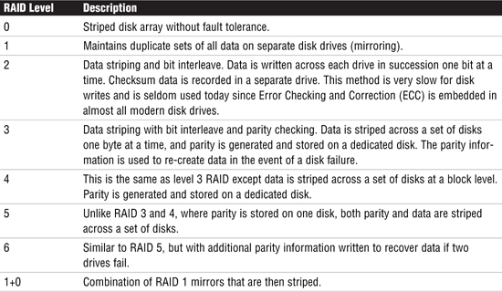
RAID level 0 does not provide data redundancy, but is usually included as a RAID classification because it is the basis for the majority of RAID configurations in use. Table 10.1 described some of the more popular RAID levels; however, many are not provided in SVM. The following is a more in-depth description of the RAID levels provided in SVM.
Exam Alert
RAID Levels For the exam, you should be familiar with RAID levels 0, 1, 5, and 1+0. These are the only levels that can be used with Solaris Volume Manager.
Although they do not provide redundancy, stripes and concatenations are often referred to as RAID 0. With striping, data is spread across relatively small, equally sized fragments that are allocated alternately and evenly across multiple physical disks. Any single drive failure can cause the volume to fail and could result in data loss. RAID 0, especially true with stripes, offers a high data transfer rate and high I/O throughput, but suffers lower reliability and availability than a single disk.
RAID 1 employs data mirroring to achieve redundancy. Two copies of the data are created and maintained on separate disks, each containing a mirror image of the other. RAID 1 provides an opportunity to improve performance for reads because read requests will be directed to the mirrored copy if the primary copy is busy. RAID 1 is the most expensive of the array implementations because the data is duplicated. In the event of a disk failure, RAID 1 provides the highest performance because the system can switch automatically to the mirrored disk with minimal impact on performance and no need to rebuild lost data.
RAID 5 provides data striping with distributed parity. RAID 5 does not have a dedicated parity disk, but instead interleaves both data and parity on all disks. In RAID 5, the disk access arms can move independently of one another. This enables multiple concurrent accesses to the multiple physical disks, thereby satisfying multiple concurrent I/O requests and providing higher transaction throughput. RAID 5 is best suited for random access data in small blocks. There is a “write penalty” associated with RAID 5. Every write I/O will result in four actual I/O operations, two to read the old data and parity and two to write the new data and parity.
Objective:
Analyze and explain SVM concepts (logical volumes, soft partitions, state databases, hot spares, and hot spare pools).
![]() Create the state database, build a mirror, and unmirror the root file system.
Create the state database, build a mirror, and unmirror the root file system.
SVM, formerly called Solstice DiskSuite, comes bundled with the Solaris 10 operating system and uses virtual disks, called volumes, to manage physical disks and their associated data. A volume is functionally identical to a physical disk from the point of view of an application. You may also hear volumes referred to as virtual or pseudo devices.
A recent feature of SVM is soft partitions. This breaks the traditional eight-slices-per-disk barrier by allowing disks, or logical volumes, to be subdivided into many more partitions. One reason for doing this might be to create more manageable file systems, given the ever-increasing capacity of disks.
Note
SVM Terminology If you are familiar with Solstice DiskSuite, you’ll remember that virtual disks were called metadevices. SVM uses a special driver, called the metadisk driver, to coordinate I/O to and from physical devices and volumes, enabling applications to treat a volume like a physical device. This type of driver is also called a logical, or pseudo driver.
In SVM, volumes are built from standard disk slices that have been created using the format utility. Using either the SVM command-line utilities or the graphical user interface of the Solaris Management Console (SMC), the system administrator creates each device by executing commands or dragging slices onto one of four types of SVM objects: volumes, disk sets, state database replicas, and hot spare pools. These elements are described in Table 10.2.

The types of SVM volumes you can create using Solaris Management Console or the SVM command-line utilities are concatenations, stripes, concatenated stripes, mirrors, and RAID 5 volumes. All of the SVM volumes are described in the following sections.
Note
No more Transactional Volumes As of Solaris 10, you should note that transactional volumes are no longer available with the Solaris Volume Manager (SVM). Use UFS logging to achieve the same functionality.
Concatenations work much the same way the Unix cat command is used to concatenate two or more files to create one larger file. If partitions are concatenated, the addressing of the component blocks is done on the components sequentially, which means that data is written to the first available slice until it is full, then moves to the next available slice. The file system can use the entire concatenation, even though it spreads across multiple disk drives. This type of volume provides no data redundancy, and the entire volume fails if a single slice fails. A concatenation can contain disk slices of different sizes because they are merely joined together.
A stripe is similar to a concatenation, except that the addressing of the component blocks is interlaced on all of the slices comprising the stripe rather than sequentially. In other words, all disks are accessed at the same time in parallel. Striping is used to gain performance. When data is striped across disks, multiple controllers can access data simultaneously. An interlace refers to a grouped segment of blocks on a particular slice, the default value being 16K. Different interlace values can increase performance. For example, with a stripe containing five physical disks, if an I/O request is, say, 64K, then four chunks of data (16K each because of the interlace size) will be read simultaneously due to each sequential chunk residing on a separate slice.
The size of the interlace can be configured when the slice is created and cannot be modified afterward without destroying and recreating the stripe. In determining the size of the interlace, the specific application must be taken into account. If, for example, most of the I/O requests are for large amounts of data, say 10 Megabytes, then an interlace size of 2 Megabytes produces a significant performance increase when using a five disk stripe. You should note that, unlike a concatenation, the components making up a stripe must all be the same size.
A concatenated stripe is a stripe that has been expanded by concatenating additional striped slices.
A mirror is composed of one or more stripes or concatenations. The volumes that are mirrored are called submirrors. SVM makes duplicate copies of the data located on multiple physical disks, and presents one virtual disk to the application. All disk writes are duplicated; disk reads come from one of the underlying submirrors. A mirror replicates all writes to a single logical device (the mirror) and then to multiple devices (the submirrors) while distributing read operations. This provides redundancy of data in the event of a disk or hardware failure.
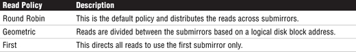
There are some mirror options that can be defined when the mirror is initially created, or following the setup. The options allow, for example, all reads to be distributed across the submirror components, improving the read performance. Table 10.3 describes the mirror read policies that can be configured.
Write performance can also be improved by configuring writes to all submirrors simultaneously. The trade-off with this option, however, is that all submirrors will be in an unknown state if a failure occurs. Table 10.4 describes the write policies that can be configured for mirror volumes.

If a submirror goes offline, it must be resynchronized when the fault is resolved and it returns to service.
Exam Alert
Read and Write Policies Make sure you are familiar with the policies for both read and write as there have been exam questions that ask for the valid mirror policies.
A RAID 5 volume stripes the data, as described in the “Stripes” section earlier, but in addition to striping, RAID 5 replicates data by using parity information. In the case of missing data, the data can be regenerated using available data and the parity information. A RAID 5 metadevice is composed of multiple slices. Some space is allocated to parity information and is distributed across all slices in the RAID 5 metadevice. The striped metadevice performance is better than the RAID 5 metadevice because the RAID 5 metadevice has a parity overhead, but merely striping doesn’t provide data protection (redundancy).
When designing your storage configuration, keep the following guidelines in mind:
![]() Striping generally has the best performance, but it offers no data protection. For write-intensive applications, RAID 1 generally has better performance than RAID 5.
Striping generally has the best performance, but it offers no data protection. For write-intensive applications, RAID 1 generally has better performance than RAID 5.
![]() RAID 1 and RAID 5 volumes both increase data availability, but they both generally result in lower performance, especially for write operations. Mirroring does improve random read performance.
RAID 1 and RAID 5 volumes both increase data availability, but they both generally result in lower performance, especially for write operations. Mirroring does improve random read performance.
![]() RAID 5 requires less disk space, therefore RAID 5 volumes have a lower hardware cost than RAID 1 volumes. RAID 0 volumes have the lowest hardware cost.
RAID 5 requires less disk space, therefore RAID 5 volumes have a lower hardware cost than RAID 1 volumes. RAID 0 volumes have the lowest hardware cost.
![]() Identify the most frequently accessed data, and increase access bandwidth to that data with mirroring or striping.
Identify the most frequently accessed data, and increase access bandwidth to that data with mirroring or striping.
![]() Both stripes and RAID 5 volumes distribute data across multiple disk drives and help balance the I/O load.
Both stripes and RAID 5 volumes distribute data across multiple disk drives and help balance the I/O load.
![]() Use available performance monitoring capabilities and generic tools such as the
Use available performance monitoring capabilities and generic tools such as the iostat command to identify the most frequently accessed data. Once identified, the “access bandwidth” to this data can be increased using striping.
![]() A RAID 0 stripe’s performance is better than that of a RAID 5 volume, but RAID 0 stripes do not provide data protection (redundancy).
A RAID 0 stripe’s performance is better than that of a RAID 5 volume, but RAID 0 stripes do not provide data protection (redundancy).
![]() RAID 5 volume performance is lower than stripe performance for write operations because the RAID 5 volume requires multiple I/O operations to calculate and store the parity.
RAID 5 volume performance is lower than stripe performance for write operations because the RAID 5 volume requires multiple I/O operations to calculate and store the parity.
![]() For raw random I/O reads, the RAID 0 stripe and the RAID 5 volume are comparable. Both the stripe and RAID 5 volume split the data across multiple disks, and the RAID 5 volume parity calculations aren’t a factor in reads except after a slice failure.
For raw random I/O reads, the RAID 0 stripe and the RAID 5 volume are comparable. Both the stripe and RAID 5 volume split the data across multiple disks, and the RAID 5 volume parity calculations aren’t a factor in reads except after a slice failure.
![]() For raw random I/O writes, a stripe is superior to RAID 5 volumes.
For raw random I/O writes, a stripe is superior to RAID 5 volumes.
Exam alert
RAID Solutions You might get an exam question that describes an application and then asks which RAID solution would be best suited for it. For example, a financial application with mission-critical data would require mirroring to provide the best protection for the data, whereas a video editing application would require striping for the pure performance gain. Make sure you are familiar with the pros and cons of each RAID solution.
Using SVM, you can utilize volumes to provide increased capacity, higher availability, and better performance. In addition, the hot spare capability provided by SVM can provide another level of data availability for mirrors and RAID 5 volumes. Hot spares were described earlier in this chapter.
After you have set up your configuration, you can use Solaris utilities such as iostat, metastat, and metadb to report on its operation. The iostat utility is used to provide information on disk usage and will show you which metadevices are being heavily utilized, while the metastat and metadb utilities provide status information on the metadevices and state databases, respectively. As an example, the output shown below provides information from the metastat utility whilst two mirror metadevices are being synchronized:

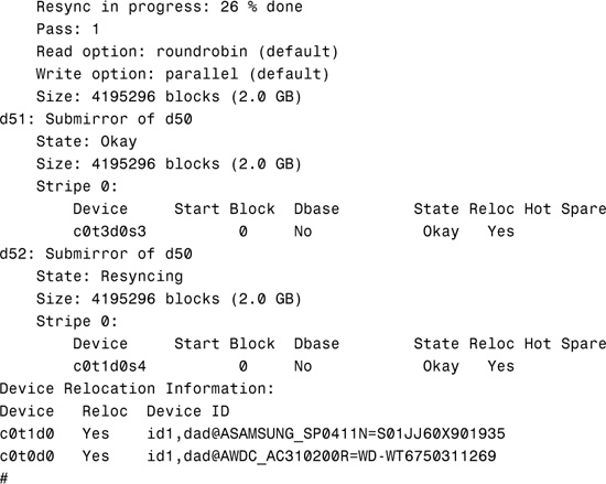
Notice from the preceding output that there are two mirror metadevices, each containing two submirror component metadevices—d60 contains submirrors d61 and d62, and d50 contains submirrors d51 and d52. It can be seen that the metadevices d52 and d62 are in the process of resynchronization. Use of this utility is important as there could be a noticeable degradation of service during the resynchronization operation on these volumes, which can be closely monitored as metastat also displays the progress of the operation, in percentage complete terms. Further information on these utilities is available from the online manual pages.
You can also use SVM’s Simple Network Management Protocol (SNMP) trap generating daemon to work with a network monitoring console to automatically receive SVM error messages. Configure SVM’s SNMP trap to trap the following instances:
![]() A RAID 1 or RAID 5 subcomponent goes into “needs maintenance” state. A disk failure or too many errors would cause the software to mark the component as “needs maintenance.”
A RAID 1 or RAID 5 subcomponent goes into “needs maintenance” state. A disk failure or too many errors would cause the software to mark the component as “needs maintenance.”
![]() A hot spare volume is swapped into service.
A hot spare volume is swapped into service.
![]() A hot spare volume starts to resynchronize.
A hot spare volume starts to resynchronize.
![]() A hot spare volume completes resynchronization.
A hot spare volume completes resynchronization.
![]() A mirror is taken offline.
A mirror is taken offline.
![]() A disk set is taken by another host and the current host panics.
A disk set is taken by another host and the current host panics.
The system administrator is now able to receive, and monitor, messages from SVM when an error condition or notable event occurs. All operations that affect SVM volumes are managed by the metadisk driver, which is described in the next section.
The metadisk driver, the driver used to manage SVM volumes, is implemented as a set of loadable pseudo device drivers. It uses other physical device drivers to pass I/O requests to and from the underlying devices. The metadisk driver operates between the file system and application interfaces and the device driver interface. It interprets information from both the UFS or applications and the physical device drivers. After passing through the metadevice driver, information is received in the expected form by both the file system and the device drivers. The metadevice is a loadable device driver, and it has all the same characteristics as any other disk device driver.
The volume name begins with “d” and is followed by a number. By default, there are 128 unique metadisk devices in the range of 0 to 127. Additional volumes, up to 8192, can be added to the kernel by editing the /kernel/drv/md.conf file. The meta block device accesses the disk using the system’s normal buffering mechanism. There is also a character (or raw) device that provides for direct transmission between the disk and the user’s read or write buffer. The names of the block devices are found in the /dev/md/dsk directory, and the names of the raw devices are found in the /dev/md/rdsk directory. The following is an example of a block and raw logical device name for metadevice d0:
![]()
You must have root access to administer SVM or have equivalent privileges granted through RBAC. (RBAC is described in Chapter 11, “Controlling Access and Configuring System Messaging.”)
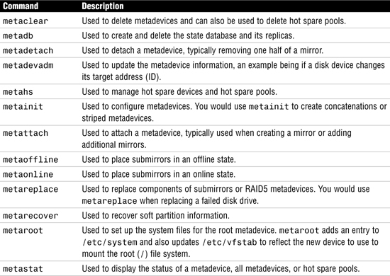
There are a number of SVM commands that will help you create, monitor, maintain and remove metadevices. All the commands are delivered with the standard Solaris 10 Operating Environment distribution. Table 10.5 briefly describes the function of the more frequently used commands that are available to the system administrator.
Note
Where They Live The majority of the SVM commands reside in the /usr/sbin directory, although you should be aware that metainit, metadb, metastat, metadevadm, and metarecover reside in /sbin—there are links to these commands in /usr/sbin as well.
Note
No More metatool You should note that the metatool command is no longer available in Solaris 10. Similar functionality—managing metadevices through a graphical utility—can be achieved using the Solaris Management Console (SMC), specifically the Enhanced Storage section.
The SVM state database contains vital information on the configuration and status of all volumes, hot spares, and disk sets. There are normally multiple copies of the state database, called replicas, and it is recommended that state database replicas be located on different physical disks, or even different controllers if possible, to provide added resilience.
The state database, together with its replicas, guarantees the integrity of the state database by using a majority consensus algorithm. The algorithm used by SVM for database replicas is as follows:
![]() The system will continue to run if at least half of the state database replicas are available.
The system will continue to run if at least half of the state database replicas are available.
![]() The system will panic if fewer than half of the state database replicas are available.
The system will panic if fewer than half of the state database replicas are available.
![]() The system cannot reboot into multi-user mode unless a majority (half+1) of the total number of state database replicas are available.
The system cannot reboot into multi-user mode unless a majority (half+1) of the total number of state database replicas are available.
Note
No Automatic Problem Detection The SVM software does not detect problems with state database replicas until there is a change to an existing SVM configuration and an update to the database replicas is required. If insufficient state database replicas are available, you’ll need to boot to single-user mode, and delete or replace enough of the corrupted or missing database replicas to achieve a quorum.
If a system crashes and corrupts a state database replica then the majority of the remaining replicas must be available and consistent; that is, half + 1. This is why at least three state database replicas must be created initially to allow for the majority algorithm to work correctly.
You also need to put some thought into the placement of your state database replicas. The following are some guidelines:
![]() When possible, create state database replicas on a dedicated slice that is at least 4MB in size for each database replica that it will store.
When possible, create state database replicas on a dedicated slice that is at least 4MB in size for each database replica that it will store.
![]() You cannot create state database replicas on slices containing existing file systems or data.
You cannot create state database replicas on slices containing existing file systems or data.
![]() When possible, place state database replicas on slices that are on separate disk drives. If possible, use drives that are on different host bus adapters.
When possible, place state database replicas on slices that are on separate disk drives. If possible, use drives that are on different host bus adapters.
![]() When distributing your state database replicas, follow these rules:
When distributing your state database replicas, follow these rules:
![]() Create three replicas on one slice for a system with a single disk drive. Realize, however, if the drive fails, all your database replicas will be unavailable and your system will crash.
Create three replicas on one slice for a system with a single disk drive. Realize, however, if the drive fails, all your database replicas will be unavailable and your system will crash.
![]() Create two replicas on each drive for a system with two to four disk drives.
Create two replicas on each drive for a system with two to four disk drives.
![]() Create one replica on each drive for a system with five or more drives.
Create one replica on each drive for a system with five or more drives.
The state database and its replicas are managed using the metadb command. The syntax of this command is
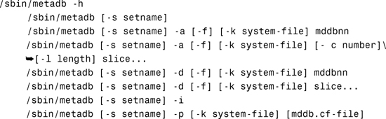
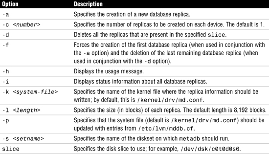
Table 10.6 describes the options available for the metadb command.
In the following example, I have reserved a slice (slice 4) on each of two disks to hold the copies of the state database, and I’ll create two copies in each reserved disk slice, giving a total of four state database replicas. In this scenario, the failure of one disk drive will result in a loss of more than half of the operational state database replicas, but the system will continue to function. The system will panic only when more than half of the database replicas are lost. For example, if I had created only three database replicas and the drive containing two of the replicas fails, the system will panic.
To create the state database and its replicas, using the reserved disk slices, enter the following command:
# metadb -a -f -c2 c0t0d0s4 c0t1d0s4
Here, -a indicates a new database is being added, -f forces the creation of the initial database, -c2 indicates that two copies of the database are to be created, and the two cxtxdxsx entries describe where the state databases are to be physically located. The system returns the prompt; there is no confirmation that the database has been created.
The following example demonstrates how to remove the state database replicas from two disk slices, namely c0t0d0s4 and c0t1d0s4:
# metadb -d c0t0d0s4 c0t1d0s4
The next section shows how to verify the status of the state database.
When the state database and its replicas have been created, you can use the metadb command, with no options, to see the current status. If you use the -i flag then you will also see a description of the status flags.
Examine the state database as shown here:

Each line of output is divided into the following fields:
![]()
flags—This field will contain one or more state database status letters. A normal status is a “u” and indicates that the database is up-to-date and active. Uppercase status letters indicate a problem and lowercase letters are informational only.
![]()
first blk—The starting block number of the state database replica in its partition. Multiple state database replicas in the same partition will show different starting blocks.
![]()
block count—The size of the replica in disk blocks. The default length is 8192 blocks (4MB), but the size could be increased if you anticipate creating more than 128 metadevices, in which case, you would need to increase the size of all state databases.
The last field in each state database listing is the path to the location of the state database replica.
As the code shows, there is one master replica; all four replicas are active and up to date and have been read successfully.
SVM requires that at least half of the state database replicas must be available for the system to function correctly. When a disk fails or some of the state database replicas become corrupt, they must be removed with the system at the Single User state, to allow the system to boot correctly. When the system is operational again (albeit with fewer state database replicas), additional replicas can again be created.
The following example shows a system with two disks, each with two state database replicas on slices c0t0d0s7 and c0t1d0s7.
If we run metadb -i, we can see that the state database replicas are all present and working correctly:

Subsequently, a disk failure or corruption occurs on the disk c0t1d0 and renders the two replicas unusable. The metadb -i command shows that there are write errors on the two replicas on c0t1d0s7:

When the system is rebooted, the following messages appear:
Insufficient metadevice database replicas located.
Use metadb to delete databases which are broken.
Ignore any Read-only file system error messages.
Reboot the system when finished to reload the metadevice database.
After reboot, repair any broken database replicas which were deleted.
To repair the situation, you will need to be in single-user mode, so boot the system with -s and then remove the failed state database replicas on c0t1d0s7.
# metadb -d c0t1d0s7
Now reboot the system again—it will boot with no problems, although you now have fewer state database replicas. This will enable you to repair the failed disk and re-create the metadevice state database replicas.
You create a simple volume when you want to place an existing file system under SVM control. The command to create a simple volume is metainit. Here is the syntax for metainit:
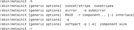
Table 10.7 describes the options available for the metainit command.

In the following example, a simple concatenation metadevice will be created using the disk slice /dev/dsk/c0t0d0s5. The metadevice will be named d100:
# metainit -f d100 1 1 c0t0d0s5
d100: Concat/Stripe is setup
Solaris Volume Manager provides the metastat command to monitor the status of all volumes. The syntax of this command is as follows:
![]()
Table 10.8 describes the options for the metastat command.

In the following example, the metastat command is used to display the status of a single metadevice, d100:
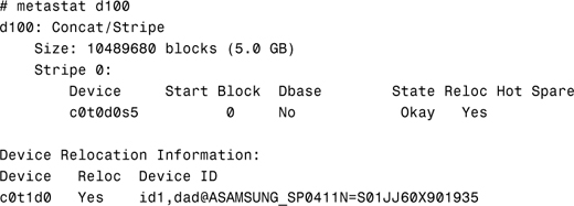
In the next example, the metastat -c command displays the status for the same metadevice (d100), but this time in concise format:
![]()
Soft partitions are used to divide large partitions into smaller areas, or extents, without the limitations imposed by hard slices. The soft partition is created by specifying a start block and a block size. Soft partitions differ from hard slices created using the format command because soft partitions can be non-contiguous, whereas a hard slice is contiguous. Therefore, soft partitions can cause I/O performance degradation.
A soft partition can be built on a disk slice or another SVM volume, such as a concatenated device. You’ll create soft partitions using the SVM command metainit. For example, let’s say that we have a hard slice named c2t1d0s1 that is 10GB in size and was created using the format command. To create a soft partition named d10 which is 1GB in size, and assuming that you’ve already created the required database replicas, issue the following command:
# metainit d10 -p c2t1d0s1 1g
The system responds with
d10: Soft Partition is setup
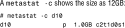
View the soft partition using the metastat command:

Create a file system on the soft partition using the newfs command as follows:
# newfs /dev/md/rdsk/d10
Now you can mount a directory named /data onto the soft partition as follows:
# mount /dev/md/dsk/d10 /data
To remove the soft partition named d10, unmount the file system that is mounted to the soft partition and issue the metaclear command as follows:
# metaclear d10
Caution
Removing the soft partition destroys all data that is currently stored on that partition.
The system responds with
d10: Soft Partition is cleared
With SVM, you can increase the size of a file system while it is active and without unmounting the file system. The process of expanding a file system consists of first increasing the size of the SVM volume, and then growing the file system that has been created on the partition. In Step by Step 10.1, I’ll increase the size of a soft partition and the file system mounted on it.
STEP BY STEP
10.1 Increasing the Size of a Mounted File System
1. Check the current size of the /data file system, as follows:
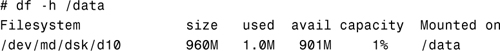
Note that the size of /data is currently 960MB.
2. Use the metattach command to increase the SVM volume named d10 from 1GB to 2GB as follows:
# metattach d10 1gb
Another metastat -c shows that the soft partition is now 2GB, as follows:
![]()
Check the size of /data again, and note that the size did not change:
![]()
3. To increase the mounted file system /data, use the growfs command as follows:

Another df -h /data command shows that the /data file system has been increased as follows:
![]()
Soft partitions can be built on top of concatenated devices, and you can increase a soft partition as long as there is room on the underlying metadevice. For example, you can’t increase a 1GB soft partition if the metadevice on which it is currently built is only 1GB in size. However, you could add another slice to the underlying metadevice d9.
In Step by Step 10.2 we will create an SVM device on c2t1d0s1 named d9 that is 4GB in size. We then will create a 3GB soft partition named d10 built on this device. To add more space to d10, we first need to increase the size of d9, and the only way to accomplish this is to add more space to d9, as described in the Step by Step.
STEP BY STEP
10.2 Concatenate a New Slice to an Existing Slice
1. Log in as root and create metadbs as described earlier in this chapter.
2. Use the metainit command to create a simple SVM volume on c2t1d0s1 as follows:
![]()
Use the metastat command to view the simple metadevice named d9 as follows:

![]()
3. Create a 3GB soft partition on top of the simple device as follows:
![]()
4. Before we can add more space to d10, we first need to add more space to the simple volume by concatenating another 3.9GB slice (c2t2d0s1) to d9 as follows:
![]()
The metastat command shows the following information about d9:
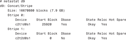

Notice that the metadevice d9 is made up of two disk slices (c2t1d0s1 and c2t2d0s1) and that the total size of d9 is now 7.9GB.
5. Now we can increase the size of the metadevice d10 using the metattach command described in Step by Step 10.1.
A mirror is a logical volume that consists of more than one metadevice, also called a submirror. In this example, there are two physical disks: c0t0d0 and c0t1d0. Slice 5 is free on both disks, which will comprise the two submirrors, d12 and d22. The logical mirror will be named d2; it is this device that will be used when a file system is created. Step by Step 10.3 details the whole process:
STEP BY STEP
10.3 Creating a Mirror
1. Create the two simple metadevices that will be used as submirrors first.
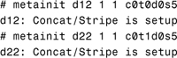
2. Having created the submirrors, now create the actual mirror device, d2, but only attach one of the submirrors—the second submirror will be attached manually.
![]()
At this point, a one-way mirror has been created.
3. Now attach the second submirror to the mirror device, d2.
![]()
At this point, a two-way mirror has been created and the second submirror will be synchronized with the first submirror to ensure they are both identical.
Caution
It is not recommended to create a mirror device and specify both submirrors on the command line, because even though it will work, there will not be a resynchronization between the two submirrors, which could lead to data corruption.
4. Verify that the mirror has been created successfully and that the two submirrors are being synchronized.
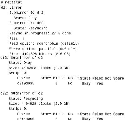
Notice that the status of d12, the first submirror, is Okay, and that the second submirror, d22, is currently resyncing, and is 27% complete. The mirror is now ready for use as a file system.
5. Create a UFS file system on the mirrored device:

Note that it is the d2 metadevice that has the file system created on it.
6. Run fsck on the newly created file system before attempting to mount it. This step is not absolutely necessary, but is good practice because it verifies the state of a file system before it is mounted for the first time:
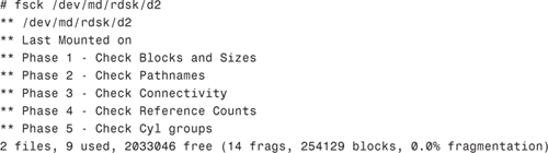
The file system can now be mounted in the normal way. Remember to edit /etc/vfstab to make the mount permanent. Remember to use the md device and for this example, we’ll mount the file system on /mnt.
# mount /dev/md/dsk/d2 /mnt
#
This section details the procedure for removing a mirror on a file system that can be removed and remounted without having to reboot the system. Step by Step 10.4 shows how to achieve this. This example uses a file system, /test, that is currently mirrored using the metadevice, d2; a mirror that consists of d12 and d22. The underlying disk slice for this file system is /dev/dsk/c0t0d0s5:
STEP BY STEP
10.4 Unmirror a Non-Critical File System
1. nmount the /test file system.
# umount /test
2. Detach the submirror, d12, that is going to be used as a UFS file system.
![]()
3. Delete the mirror (d2) and the remaining submirror (d22).
![]()
At this point, the file system is no longer mirrored. It is worth noting that the metadevice, d12, still exists and can be used as the device to mount the file system. Alternatively, the full device name, /dev/dsk/c0t0d0s5, can be used if you do not want the disk device to support a volume. For this example, we will mount the full device name (as you would a normal UFS file system), so we will delete the d12 metadevice first.
4. Delete the d12 metadevice:
![]()
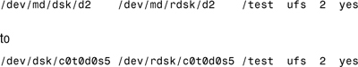
5. Edit /etc/vfstab to change the entry:
6. Remount the /test file system:
# mount /test
In this section we will create another mirror, but this time it will be the root file system. This is different from Step by Step 10.3 because we are mirroring an existing file system that cannot be unmounted. We can’t do this while the file system is mounted, so we’ll configure the metadevice and a reboot will be necessary to implement the logical volume and to update the system configuration file. The objective is to create a two-way mirror of the root file system, currently residing on /dev/dsk/c0t0d0s0. We will use a spare disk slice of the same size, /dev/dsk/c0t1d0s0, for the second submirror. The mirror will be named d0, and the submirrors will be d10 and d20. Additionally, because this is the root (/) file system, we’ll also configure the second submirror as an alternate boot device, so that this second slice can be used to boot the system if the primary slice becomes unavailable. Step by Step 10.5 shows the procedure to follow:
STEP BY STEP
10.5 Mirror the root File System
1. Verify that the current root file system is mounted from /dev/dsk/c0t0d0s0.
![]()
2. Create the state database replicas, specifying the disk slices c0t0d0s4 and c0t0d0s5. We will be creating two replicas on each slice.
![]()
3. Create the two submirrors, d10 and d20.
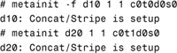
Note that the -f option was used in the first metainit command. This is the option to force the execution of the command, because we are creating a metadevice on an existing, mounted file system. The -f option was not necessary in the second metainit command because the slice is currently unused.
4. Create a one-way mirror, d0, specifying d10 as the submirror to attach.
![]()
5. Set up the system files to support the new metadevice, after taking a backup copy of the files that will be affected. It is a good idea to name the copies with a relevant extension, so that they can be easily identified if you later have to revert to the original files, if problems are encountered. We will use the .nosvm extension in this step by step.
![]()
The metaroot command has added the following lines to the system configuration file, /etc/system, to allow the system to boot with the / file system residing on a logical volume. This command is only necessary for the root device.
![]()
It has also modified the /etc/vfstab entry for the / file system. It now reflects the metadevice to use to mount the file system at boot time:
![]()
6. Synchronize file systems prior to rebooting the system.
# lockfs -fa
The lockfs command is used to flush all buffers so that when the system is rebooted, the file systems are all up to date. This step is not compulsory, but is good practice.
7. Reboot the system.
# init 6
8. Verify that the root file system is now being mounted from the metadevice /dev/md/dsk/d0.
![]()
9. The next step is to attach the second submirror and verify that a resynchronization operation is carried out.

10. Install a boot block on the second submirror to make this slice bootable. This step is necessary because it is the root (/) file system that is being mirrored.
![]()
The uname -I command substitutes the system’s platform name.
11. Identify the physical device name of the second submirror. This will be required to assign an OpenBoot alias for a backup boot device.

Record the address starting with /pci... and change the dad string to disk, leaving you, in this case, with /pci@1f,0/pci@1,1/ide@3/disk@1,0:a.
12. For this step you need to be at the ok prompt, so enter init 0 to shut down the system.
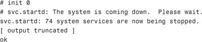
Enter the nvalias command to create an alias named backup - root, which points to the address recorded in step 11.
![]()
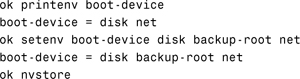
Now inspect the current setting of the boot-device variable and add the name backup-root as the secondary boot path, so that this device is used before going to the network. When this has been done, enter the nvstore command to save the alias created.
13. The final step is to boot the system from the second submirror to prove that it works. This can be done manually from the ok prompt, as follows:

Unlike Step by Step 10.4, where a file system was unmirrored and remounted without affecting the operation of the system, unmirroring a root file system is different because it cannot be unmounted while the system is running. In this case, it is necessary to perform a reboot to implement the change. Step by Step 10.6 shows how to unmirror the root file system that was successfully mirrored in Step by Step 10.5. This example comprises a mirror, d0, consisting of two submirrors, d10 and d20. The objective is to remount the / file system using its full disk device name, /dev/dsk/c0t0d0s0, instead of using /dev/md/dsk/d0:
STEP BY STEP
10.6 Unmirror the root File System
1. Verify that the current root file system is mounted from the metadevice /dev/md/dsk/d0.
![]()
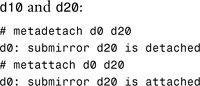
2. Detach the submirror that is to be used as the / file system.
![]()
3. Set up the /etc/system file and /etc/vfstab to revert to the full disk device name,
![]()
Notice that the entry that was added to /etc/system when the file system was mirrored has been removed, and that the /etc/vfstab entry for / has reverted back to /dev/dsk/c0t0d0s0.
4. Reboot the system to make the change take effect.
# init 6
5. Verify that the root file system is now being mounted from the full disk device,
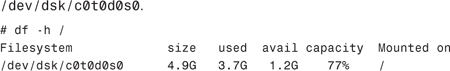
6. Remove the mirror, d0, and its remaining submirror, d20.
![]()
7. Finally, remove the submirror, d10, that was detached earlier in step 2.
![]()
Occasionally, a root mirror fails and recovery action has to be taken. Often, only one side of the mirror fails, in which case it can be detached using the metadetach command. You then replace the faulty disk and reattach it. Sometimes though, a more serious problem occurs prohibiting you from booting the system with SVM present. In this case, you have two options available to you. First, temporarily remove the SVM configuration so that you boot from the original c0t0d0s0 device, or second, you boot from a CD-ROM and recover the root file system manually, by carrying out an fsck.
To disable SVM, you must reinstate pre-SVM copies of the files /etc/system and /etc/vfstab. In Step by Step 10.5 we took a copy of these files (step 5). This is good practice and should always be done when editing important system files. Copy these files again, to take a current backup, and then copy the originals back to make them operational, as shown here:
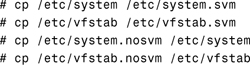
You should now be able to reboot the system to single-user without SVM and recover any failed file systems.
If the preceding does not work, it might be necessary to repair the root file system manually, requiring you to boot from a CD-ROM. Insert the Solaris 10 CD 1 disk (or the Solaris 10 DVD) and shut down the system if it is not already shut down.
Boot to single-user from the CD-ROM as follows:
ok boot cdrom -s
When the system prompt is displayed, you can manually run fsck on the root file system. In this example, I am assuming a root file system exists on /dev/rdsk/c0t0d0s0:

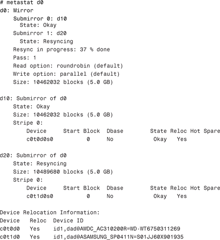
You should now be able to reboot the system using SVM and you should resynchronize the root mirror as soon as the system is available. This can be achieved easily by detaching the second submirror and then reattaching it. The following example shows a mirror d0 consisting of
To demonstrate that the mirror is performing a resynchronization operation, you can issue the metastat command as follows, which will show the progress as a percentage:
Exam Alert
Veritas Volume Manager There are no questions on the Veritas Volume Manager in the exam. This section has been included solely to provide some additional information for system administrators and to allow comparison between this product and the Solaris Volume Manager. A course is run by Sun Microsystems for administrators using Veritas Volume Manager.
Veritas Volume Manager is an unbundled software package that can be purchased separately via Sun, or direct from Veritas, and does not come as part of the standard Solaris 10 release. This product has traditionally been used for managing Sun’s larger StorEdge disk arrays. It is widely used for performing Virtual Volume Management functions on large scale systems such as Sun, Sequent, and HP. Although Veritas Volume Manager also provides the capability to mirror the OS drive, in actual industry practice, you’ll still see SVM used to mirror the OS drive, even on large Sun servers that use Veritas Volume Manager to manage the remaining data. It used to be much more robust than the older Solstice DiskSuite product—the predecessor to the Solaris Volume Manager, providing tools that identify and analyze storage access patterns so that I/O loads can be balanced across complex disk configurations. SVM is now a much more robust product but the difference is negligible.
Veritas Volume Manager is a complex product that would take much more than this chapter to describe in detail. This chapter will, however, introduce you to the Veritas Volume Manager and some of the terms you will find useful.
The Volume Manager builds virtual devices called volumes on top of physical disks. A physical disk is the underlying storage device (media), which may or may not be under Volume Manager control. A physical disk can be accessed using a device name such as /dev/rdsk/c#t#d. The physical disk, as explained in Chapter 1, can be divided into one or more slices.
Volumes are accessed by the Solaris file system, a database, or other applications in the same way physical disk partitions would be accessed. Volumes and their virtual components are referred to as Volume Manager objects.
There are several Volume Manager objects that the Volume Manager uses to perform disk management tasks (see Table 10.9).

Note
Plex Configuration A number of plexes (usually two) are associated with a volume to form a working mirror. Also, stripes and concatenations are normally achieved during the creation of the plex.
Volume Manager objects can be manipulated in a variety of ways to optimize performance, provide redundancy of data, and perform backups or other administrative tasks on one or more physical disks without interrupting applications. As a result, data availability and disk subsystem throughput are improved.
Veritas Volume Manager manages disk space by using contiguous sectors. The application formats the disks into only two slices: Slice 3 and Slice 4. Slice 3 is called a private area and Slice 4 is the public area. Slice 3 maintains information about the virtual to physical device mappings, while Slice 4 provides space to build the virtual devices. The advantage to this approach is that there is almost no limit to the number of subdisks you can create on a single drive. In a standard Solaris disk partitioning environment, there is an eight-partition limit per disk.
The names of the block devices for virtual volumes created using Veritas Volume Manager are found in the /dev/vx/dsk/<disk_group>/<volume_name> directory, and the names of the raw devices are found in the /dev/vx/rdsk/<disk_group>/<volume_name> directory. The following is an example of a block and raw logical device name:
![]()
This chapter described the basic concepts behind RAID and the Solaris Volume Manager (SVM). This chapter described the various levels of RAID along with the differences between them, as well as the elements of SVM and how they can be used to provide a reliable data storage solution. We also covered the creation and monitoring of the state database replicas and how to mirror and unmirror file systems. Finally, you learned about Veritas Volume Manager, a third-party product used predominantly in larger systems with disk arrays.
![]() Meta state database
Meta state database
![]() Veritas Volume Manager objects
Veritas Volume Manager objects
![]() Hot-pluggable
Hot-pluggable
![]() Hot-swappable
Hot-swappable
In this exercise, you’ll see how to use the iostat utility to monitor disk usage. You will need a Solaris 10 workstation with local disk storage and a file system with at least 50 Megabytes of free space. You will also need CDE window sessions. For this exercise, you do not have to make use of metadevices because the utility will display information on standard disks as well as metadevices. The commands are identical whether or not you are running Solaris Volume Manager. Make sure you have write permission to the file system.
Estimated Time: 5 minutes
1. In the first window, start the iostat utility so that extended information about each disk or metadevice can be displayed. Also, you will enter a parameter to produce output every 3 seconds. Enter the following command at the command prompt:
iostat -xn 3
2. The output will be displayed and will be updated every 3 seconds. Watch the %b column, which tells you how busy the disk, or metadevice, is at the moment.
3. In the second window, change to the directory where you have at least 50 Megabytes of free disk space and create an empty file of this size, as shown in the following code. My example directory is /data. The file to be created is called testfile.
![]()
4. The file will take several seconds to be created, but watch the output being displayed in the first window and notice the increase in the %b column of output. You should see the affected file system suddenly become a lot busier. Continue to monitor the output when the command has completed and notice that the disk returns to its normal usage level.
5. Press Ctrl+C to stop the iostat output in the first window and delete the file created when you have finished, as shown here:
rm testfile
|
1. |
B. A volume (often called a |
|
A. A mirror is composed of one or more simple metadevices called submirrors. A mirror replicates all writes to a single logical device (the mirror) and then to multiple devices (the submirrors) while distributing read operations. This provides redundancy of data in the event of a disk or hardware failure. For more information, see the “Solaris SVM” section. |
|
|
3. |
D. A stripe is similar to concatenation, except that the addressing of the component blocks is interlaced on all of the slices rather than sequentially. For more information, see the “SVM Volumes” section. |
|
4. |
C. Concatenations work in much the same way as the Unix |
|
5. |
A. The names of the block devices for virtual volumes created using Veritas Volume Manager are found in the |
|
6. |
B. A volume is a virtual disk device that appears to applications, databases, and file systems like a physical logical device, but does not have the physical limitations of a physical disk partition. For more information, see the “Veritas Volume Manager” section. |
|
7. |
A. A hot spare pool is a collection of slices (hot spares) reserved to be automatically substituted in case of slice failure in either a submirror or RAID 5 metadevice. For more information, see the “Solaris SVM” section. |
|
8. |
C. A set of contiguous disk blocks, subdisks are the basic units in which the Volume Manager allocates disk space. For more information, see the “Veritas Volume Manager” section. |
|
9. |
D. RAID 5 replicates data by using parity information. In the case of missing data, the data can be regenerated using available data and the parity information. For more information, see the “RAID” section. |
|
10. |
D. In a standard Solaris SPARC disk-partitioned environment, there is an eight-partition limit per disk. For more information, see the “Solaris SVM” section. |
|
11. |
C. The command |
|
12. |
B. The command |
1. Solaris 10 Documentation CD—”Solaris Volume Manager Administration Guide” manual.
2. http://docs.sun.com. Solaris 10 documentation set. Solaris Volume Manager Administration Guide book in the System Administration collection.