Appendix E

The Nodal Method to Calculate the Partial Inductance of Finite Ground Planes

In this appendix the nodal method for analysis in the frequency domain is introduced and applied to compute the effective partial inductance L_gnd associated with the return path of two typical trace structures in PCBs: a microstrip and a stripline with finite ground planes. This inductance is very important for Ground Loop Coupling (GLC) calculation (see Section 10.1) and radiated emission prediction (see Chapter 9). The method is validated by comparing the results with those obtained by SPICE and by the method of moments.

E.1 Nodal Method Equations

Consider a network with (N + 1) nodes (0 reference node and h = 1, 2,…,N remaining nodes) and B branches, each represented as in Figure E.1. Currents and voltages at each branch can be computed by the following equations in matrix form [1]:

where:

• and are the vectors containing respectively the independent voltage and current sources of the B branches.
• A is the reduced incident matrix of B rows and N columns. The generic element A_hk assumes the following values: 1 if node h is an initial node of branch r, −1 if node h is a final node of branch r, and 0 otherwise.

  

  Figure E.1 Generic equivalent circuit of a network branch

• and are vectors containing the voltages and currents of the B branches respectively.
• and are vectors containing the voltages and currents on the impedance of the B branches respectively.
• is the squared matrix of dimension B × B. is the admittance matrix and is the impedance matrix. and are diagonal matrices if there is no coupling between the branches. When the coupling is due to voltage-dependent current sources, some or all of the off-diagonal elements have a non-zero value equal to the value of the coupling parameter between h and k branches. For instance, in the case of mutual inductance between the branches, and 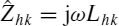, with h ≠ k, where L_hk is the mutual inductance between the hth and kth branches. When the coupling is due to current-dependent voltage sources, it is the coupling parameter that must be directly added to the off-diagonal elements of .

E.2 Nodal Method Applied to Compute the Partial Inductance Associated with a Finite Ground Plane

The Nodal Method (NM) can be very useful in signal integrity investigations when the nodal matrix contains many elements. The following example treats the computation of the partial inductance L_gnd associated with a finite ground plane of a structure composed of a plane and a conductor above the ground plane, as shown in Figure E.2. This is one of the cases presented in Section 10.1 and solved by the nodal network approach.

Figure E.2 A trace above a finite ground plane

Figure E.3 Equivalent circuit for the trace above a ground plane. The ground is divided into five sub-bars or filaments. All mutual inductances are accounted for

The geometrical dimensions of the structure under investigation (see Figure E.2) are: w_s = 0.25 mm, w_gnd = 2.5 mm, d = 0.5 mm, t = 0.1 mm. Both conductors are 1 m long. The equivalent circuit of the structure is shown in Figure E.3, where the ground plane is divided into five filaments. Therefore, there are seven branches in total: index 0 for the source, indices 1–5 for the filaments of the ground plane, and index 6 for the conductor above the ground plane.

With the orientation of the currents as indicated in Figure E.3, the matrices for computations are:

The values in matrix L are calculated by the expressions for the self partial inductance of a rectangular-cross-section conductor and the mutual inductance of two filaments, as reported in Table A.2 of Appendix A, and are expressed in H/m.

As stated in Appendix A, L_gnd is the immaginary part of the ratio between the voltage drop on the ground plane that is caused by a current flowing on the conductor above the ground and the term ωÎ. Therefore, using the elements of matrices and :

where is the second element of the voltage vector , is the first element of the current vector , and ω₀ is the angular frequency used for calculation. In the case considered, f₀ = 10 MHz. As, for simplicity, the resistances are not considered in the calculation of matrix , L_gnd is not dependent on the frequency chosen for calculation. The result of the Nodal Method is L_gnd-NM = 80.632 nH, as against the SPICE result of L_gnd-SPICE = 80.630 nH. With the approximate closed-form expression of Table A.2, L_{gnd-Analytical} = 75.1 nH.

The advantage of NM over the SPICE method consists in the fact that NM can be easily implemented in mathematical software such as MathCad or Matlab, and the number of sub-bars used to decompose the ground plane can be expanded to higher values without great effort. For instance, consider the same microstrip structure as in Figure 10.9 of Section 10.2, with w_s = 2 mm, w_gnd = 30 cm, d = 3 mm, and t = 0.1 mm for 0.3 m of conductor length. Choosing 150 filaments for the ground plane, sub-bars of width 2 mm are obtained. With these values, L_gnd-NM = 1.26 nH and L_{gnd-Analytical} = 1.16 nH. As validation of the NM, the curve of the distribution of the current density along the ground plane is very close to the distribution obtained applying the Method of Moment (MOM) (compare Figure E.4a and Figure 10.9). The quantity is the current on the trace, and is the density of current associated with the hth filament of the ground plane, where Δ = w_m/150, computed at the angular frequency ω₀.

The same computation was performed for the stripline structure of Figure 10.10. The result shown in Figure E.4b should be compared with the curve of Figure 10.10 for Δw = 0. Although the two approaches are completely different (the NM method applies the partial inductance concept, whereas the MOM method applies incident and scattered fields), the results are in very good agreement, except for some slightly different values at the edge of the planes, as the computation with MOM (see Section 10.2.1) was performed at 1 GHz. Performing computation at 1 MHz by MOM, it can be shown that there is also perfect agreement of the curves on the edges.

Figure E.4 Current density distribution computed by the Nodal Method, normalized to the total current injected into the ground plane: (a) microstrip structure; (b) stripline structure

References

[1] Adby, P.R., ‘Applied Circuit Theory: Matrix and Computer Methods’, Ellis Horwood Limited, distributed by John Wiley & Sons, Ltd, Chichester, UK, 1980.