
Using Goals in Model-Based Reasoning
Abstract
This part of Data Science for Software Engineering: Sharing Data and Models explores ensemble learners and multiobjective optimizers as applied to software engineering. Novel incremental ensemble learners are explained along with one of the largest ensemble learning (in effort estimation) experiments yet attempted. It turns out that the specific goals of the learning has an effect on what is learned and, for this reason, this part also explores multigoal reasoning. We show that multigoal optimizers can significantly improve effort estimation results.
In summary, this chapter proposes the following data analysis pattern:
| Name: | Multiobjective learning. |
| Also known as: | Pareto ensemble; multiobjective ensemble of learning machines. |
| Intent: | Software effort estimation (SEE), when one wishes to perform well in terms of different goals/objectives/performance measures. |
| Motivation: | Several performance measures can be used for evaluating the performance of SEE models. These measures can behave differently from each other [133, 389]. What is the relationship among different measures? Can we use this relationship in order to create models able to improve estimations in terms of different measures? Can we emphasize a particular measure if we wish to? |
| Solution: | SEE is formulated as a multiobjective learning problem, where different performance measures are seen as goals/objectives to be optimized. A multiobjective evolutionary algorithm (MOEA) is used to optimize on all these measures at the same time, allowing us to create an ensemble of models that provides a good trade-off among different measures (Pareto ensemble), or to emphasize particular measures. |
| Applicability: | Plots of models created by the multiobjective algorithm can be used to obtain a better understanding of the relationship among different measures. In particular, it was revealed that different measures can present even opposite behaviors. The Pareto ensemble was successful in obtaining similar or better performance than a traditional corresponding single-objective approach. Competitive performance was also obtained in comparison to several other approaches, in particular on more heterogeneous data sets [327]. |
| Related to: | Chapter 20 in terms of ensemble learning; Chapter 23 in terms of the importance of objectives/goals. |
This chapter is based on Minku and Yao [327]. Additionally, the following new material has been added: (1) a didactic explanation of multilayer perceptrons (MLPs) (Section 24.1); (2) an introduction to MOEAs and its components (Section 24.2); and (3) a didactic explanation of harmonic-distance MOEA (Section 24.3).
Much of the software prediction work involves empirical evaluation of models. Several different performance measures can be used for that. For instance, in SEE, one can use the mean magnitude of the relative error (MMRE), the percentage of estimations within N% of the actual value (PRED(N)), the logarithmic standard deviation (LSD) [133], the mean absolute error (MAE) [389], etc. Different performance measures can behave differently and it is highly unlikely that there is a “single, simple-to-use, universal goodness-of-fit kind of metric” [133], i.e., none of these measures is totally free of problems! Section 24.4.1 will explain some of these measures in more detail.
You may then be thinking: “If they are all measures of performance, why can not we just improve in all of them?” However, things are not so simple, because some of these measures may have conflicting behavior, i.e., as models are improved in one of them, they may be degraded in others. In this chapter, we show that improving on different performance measures that we are interested in can be seen as different goals/objectives when learning software prediction models. Ideally, we would indeed like to achieve all these goals. If the performance measures behave quite differently from each other on a given software prediction task, it may be possible to improve on different measures by using them as a natural way to generate diversity in ensembles.
As explained in Chapters 20, 22, ensembles have been showing relatively good performance for SEE, and diversity is a key component for their performance (Section 20.1). However, the ensemble presented in Chapter 22 requires a manual procedure for building the ensemble that focuses on improving accuracy of the base models. As there is a trade-off between accuracy and diversity of base models [69], focusing only on improving base models' accuracy may lead to lack of diversity, reducing the performance of the ensemble as a whole. The ensemble presented in Chapter 20 is automated and based on an ensemble method known to encourage diversity. However, despite the fact that it is somewhat tailored to SEE by joining the power of ensembles and locality, it is still based on general-purpose techniques. Additional improvements may be obtained by further tailoring ensembles for the task at hand [326]. Encouraging diversity based on a set of objectives specifically designed for a certain software prediction task may provide further improvements in this task. With that in mind, this chapter attempts to answer the following research questions:
• RQ1. What is the relationship among different performance measures for SEE? Despite existing studies on different performance measures [133, 215], it is still not well understood to what extend different performance measures behave differently in SEE. This is necessary in order to decide on how to use them for evaluation and model-building purposes.
• RQ2. Can we use different performance measures as a source of diversity to create SEE ensembles? In particular, can that improve the performance in comparison to models created without considering these measures explicitly? Existing models do not necessarily consider the performance measures in which we are interested explicitly. For example, MLPs are usually trained using backpropagation, which is based on the mean squared error (MSE). So, they can only improve on other performance measures indirectly. We will check whether creating an ensemble considering MMRE, PRED, and LSD explicitly leads to more improvements in the SEE context.
• RQ3. Is it possible to create SEE models that emphasize particular performance measures should we wish to do so? For example, if there is a certain measure that we believe to be more appropriate than the others, can we create a model that particularly improves performance considering this measure? This is useful not only for the case where the software manager has sufficient domain knowledge to chose a certain measure, but also (and mainly) if there are future developments of the SEE research showing that a certain measure is better than others for a certain purpose.
In order to answer these questions, we formulate the problem of creating SEE models as a multiobjective learning problem that considers different performance measures explicitly as objectives to be optimized. This formulation is key to answer the research questions because it allows us to use a MOEA [438] to generate SEE models that are generally good considering all the predefined performance measures. This feature allows us to use plots of the performances of these models in order to understand the relationship among the performance measures and how differently they behave. Once these models are obtained, the models that perform best for each different performance measure can be determined. These models behave differently from each other and can be used to form a diverse ensemble that provides an ideal trade-off among these measures. Therefore, this approach creates ensembles in such a way to encourage both accuracy and diversity, which is known to be beneficial for ensembles [61, 244]. Choosing a single performance measure is not an easy task. By using our ensemble, the software manager does not need to chose a single performance measure, as an ideal trade-off among different measures is provided. As an additional benefit of this approach, each of the models that compose the ensemble can also be used separately to emphasize a specific performance measure if desired.
The approach presented in this chapter is fully automated and tailored for SEE. Once developed, a tool using this approach can be easily run to learn models and create ensembles. It is worth noting that the parameters choice can also be automated for this approach, as long as the developer of the tool embeds on it several different parameter values to be tested on a certain percentage of the completed projects of the company being estimated.
Our analysis shows that the different performance measures MMRE, PRED, and LSD behave very differently when analyzed at their individual best level, and sometimes present even opposite behaviors (RQ1). For example, when considering nondominated (Section 24.2) solutions, as MMRE is improved, LSD tends to get worse. This is an indicator that these measures can be used to create diverse ensembles for SEE. We then show that MOEA is successful in generating SEE ensemble models by optimizing different performance measures explicitly at the same time (RQ2). The ensembles are composed of nondominated solutions selected from the last generation of the MOEA, as explained in Section 24.4. These ensembles present performance similar or better than a model that does not optimize the three measures concurrently. Furthermore, the similar or better performance is achieved considering all the measures used to create the ensemble, showing that these ensembles not only provide a better trade-off among different measures, but also improve the performance considering these measures. We also show that MOEA is flexible, allowing us to chose solutions that emphasize certain measures, if desired (RQ3).
The base models generated by the MOEA in this work are MLPs [32], which have been showing success for not being restricted to linear project data [422]. Even though we generate MLPs in this work, MOEAs could also be used to generate other types of base learners, such as radial basis function networks (RBFs), regression trees (RTs), and linear regression equations. An additional comparison of MOEA to evolve MLPs was performed against nine other approaches, involving other types of models. The comparison shows that the MOEA ensembles of MLPs were ranked first more often in terms of five different performance measures, but performed less well in terms of LSD. They were also ranked first more often for the data sets likely to be more heterogeneous. It is important to note, though, that this additional comparison is not only evaluating the MOEA and the multiobjective formulation of the problem, but also the type of model being evolved (MLP). Other types of models could also be evolved by the MOEA and could possibly provide better results in terms of LSD. As the key point of this work is to analyze the multiobjective formulation of the creation of SEE models, and not the comparison among different types of models, experimentation with different types of MOEA and different types of base models is left as future work.
This chapter is organized as follows. Section 24.1 explains MLPs. Section 24.2 explains MOEAs in general. Section 24.3 explains a particular type of MOEA. Section 24.4 explains our approach for creating SEE models (including ensembles) through MOEAs. In particular, Section 24.4.1 explains the multiobjective formulation of the problem of creating SEE models. Section 24.5 explains the experimental design for answering the research questions and evaluating our approach. Section 24.6 provides an analysis of the relationship among different performance measures (RQ1). Section 24.7 provides an evaluation of the MOEA's ability to create ensembles by optimizing several different measures at the same time (RQ2). Section 24.8 shows that MOEAs are flexible, allowing us to create models that emphasize particular performance measures, if desired (RQ3). Section 24.9 shows that there is still room for improvement in the choice of MOEA models to be used for SEE. Section 24.10 complements the evaluation by checking how well the Pareto ensemble of MLPs performs in comparison to other types of models. Section 24.11 presents a summary of the chapter.
24.1 Multilayer Perceptrons
MLPs are neural network models that work as universal approximators, i.e., they can approximate any continuous function [180]. For instance, they can be used as SEE models. MLPs are composed of neurons called perceptions. So, before explaining the general structure of MLPs, the general structure of a perceptron [372] will be explained. As shown in Figure 24.1, a perceptron receives n features as input (x = x1, x2,…, xn), and each of these features is associated to a weight. Input features must be numeric. So, nonnumeric input features have to be converted to numeric ones in order to use a perceptron. For instance, a categorical feature with p possible values can be converted into p input features representing the presence/absence of these values. These are called dummy variables. For example, if the input feature “development type” can take the values “new development,” “enhancement,” or “re-development,” it could be replaced by three dummy variables “new development,” “enhancement,” and “redevelopment,” which take value 1 if the corresponding value is present and 0 if it is absent.
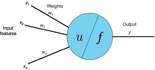
The input features are passed on to an input function u, which computes the weighted sum of the input features:
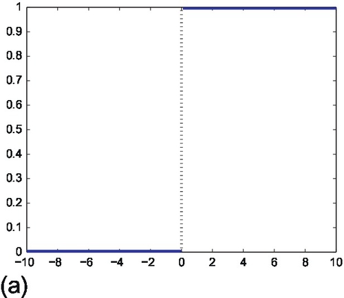
The result of this computation is then passed onto an activation function f, which will produce the output of the perceptron. In the original perceptron, the activation function is a step function:
where θ is a threshold parameter. An example of step function with θ = 0 is shown in Figure 24.2a. Thus, we can see that the perceptron determines whether w1x1 + w2x2 + ![]() + wnxn − θ > 0 is true or false. The equation w1x1 + w2x2 +
+ wnxn − θ > 0 is true or false. The equation w1x1 + w2x2 + ![]() + wnxn − θ = 0 is the equation of a hyperplane. The perceptron outputs 1 for any input point above the hyperplane, and outputs 0 for any input on or below the hyperplane. For this reason, the perceptron is called a linear classifier, i.e., it works well for data that are linearly separable. Perceptron learning consists of adjusting the weights so that a hyperplane that separates the training data well is determined. We refer the reader to Gurney [151] for more information on the perceptron's learning algorithm.
+ wnxn − θ = 0 is the equation of a hyperplane. The perceptron outputs 1 for any input point above the hyperplane, and outputs 0 for any input on or below the hyperplane. For this reason, the perceptron is called a linear classifier, i.e., it works well for data that are linearly separable. Perceptron learning consists of adjusting the weights so that a hyperplane that separates the training data well is determined. We refer the reader to Gurney [151] for more information on the perceptron's learning algorithm.

MLPs are able to approximate any continuous function, rather than only linear functions. They do so by combining several neurons, which are organized in at least three layers:
• One input layer, which simply distributes the input features to the first hidden layer.
• One or more hidden layers of perceptrons. The first hidden layer receives as inputs the features distributed by the input layer. The other hidden layers receive as inputs the output of each perceptron from the previous layer.
• One output layer of perceptrons, which receive as inputs the output of each perceptron of the last hidden layer.
Figure 24.3 shows a scheme of an MLP with three layers. The perceptrons used by MLPs frequently use other types of activation functions than the step function. For the hidden layer neurons, sigmoid functions are frequently used. An example of a sigmoid function is shown in Figure 24.2b. Sigmoid functions will lead to smooth transitions instead of hardlined decision boundaries as when using step functions. The activation function of the output layer neurons is typically sigmoid for classification problems and the identity function for regression problems.

Learning in MLPs also consists in adjusting its perceptrons' weights so as to provide low error on the training data. This is traditionally done using the backpropagation algorithm [151], which attempts to minimize the MSE. However, other algorithms can also be used. In this chapter, we will show how to use MOEAs for training MLPs based on several different performance measures. Strategies can also be used to avoid overfitting the training data, i.e., to avoid creating models that have poor predictive performance due to modeling random error or noise present in the training data. Avoiding overfitting frequently involves allowing a higher error on the training data than the one that could be achieved by the model.
24.2 Multiobjective evolutionary algorithms
Evolutionary algorithms (EAs) are optimization algorithms that search for optimal solutions by evolving a multiset1 of candidate solutions.2 MOEAs are EAs able to look for solutions that are optimal in terms of two or more possibly conflicting objectives. In the case of SEE, candidate solutions can be SEE models. So, MOEAs can be used to search for good SEE models. There exist several different types of MOEAs. Examples of MOEAs are the conventional and well-known nondominated sorting genetic algorithm II (NSGA-II) [93]; the improved strength Pareto evolutionary algorithm (SPEA2) [465]; the two-archive algorithm [362]; the indicator-based evolutionary algorithm (IBEA) [464]; and the harmonic distance MOEA (HaD-MOEA) [438].
MOEAs typically operate by following the general scheme of EAs shown in Figure 24.4. Different MOEAs differ in the way they implement the steps shown in this figure. The scheme works as follows. EAs first generate a multiset of candidate solutions randomly. This multiset of candidate solutions are then evaluated to determine their quality. A certain number of candidate solutions are selected as parents. These are candidate solutions that will be used to generate new candidate solutions. The next steps are to combine and/or modify the parents by using variation operators to generate new candidate solutions, and to evaluate these new solutions. A multiset of candidate solutions is selected to survive for the next generation, i.e., a multiset of solutions is selected to comprise the population in the next iteration of the algorithm. In the next generation, the whole procedure from parents selection onward is repeated. This repetition continues until a certain termination condition is met. This could be, for example, a predefined maximum number of generations.
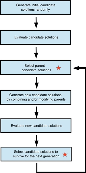
The steps marked with a Star in Figure 24.4 usually contain some selection pressure toward the selection of better solutions. In this way, as generations pass, populations are evolved toward better solutions. As MOEAs aim to optimize two or more possibly conflicting objectives, their selection pressure must consider all these objectives in some way in order to determine which solutions are “better.” This is frequently done through the concept of dominance [93], even though there are also MOEAs that operate in different ways [378]. A solution s1 dominates another solution s2 if
• s1 performs at least as well as s2 in any objective; and
• s1 performs better than s2 in at least one objective.
By using the concept of dominance, a solution s1 that dominates another solution s2 can be seen as “better” than s2. Thus, the MOEA looks for solutions that are nondominated by other solutions. The set of optimal solutions nondominated by any other solution in the search space is referred to as Pareto front. Even though the true Pareto front is very difficult to find, a MOEA can often find a set of good solutions nondominated by any other solution in the last generation. For simplicity, we will refer to the nondominated solutions in the last generation as Pareto solutions in this work.
The components of an EA are the following (please refer to Eiben and Smith [111] for more details):
• Representation: candidate solutions must be represented within the EA in such a way to allow easy manipulation by the EA without restricting areas of the search space that may contain important solutions. Solutions represented within the EA's context are called genotypes, whereas solutions in the original problem context are called phenotypes. For example, in SEE, the phenotype could be a SEE model such as an MLP, whereas the genotype could be a vector of floating point numbers representing the weights of the MLP.
• Objective/evaluation functions: these are functions that represent the requirements to improve on. In MOEAs, there is more than one objective function. For example, in the case of SEE, Section 24.4.1 shows that we can use different performance measures (e.g., MMRE, PRED(25), and LSD) calculated on the training set as objective functions. In single-objective EAs, the objective function is typically referred to as fitness function.
• Population: this is a multiset of genotypes maintained by the EA. It typically keeps a constant size as generations pass.
• Parents selection mechanism: in order to create pressure toward better candidate solutions, parents are typically selected through a probabilistic mechanism that gives higher chances for selecting better candidate solutions and smaller chances for selecting lower quality ones. The probabilistic nature of selection helps to avoid the algorithm getting stuck in local optima. An example of parents selection mechanism is binary tournament selection [317]. In this case, two candidate solutions are picked uniformly at random from the population, and the best between them is selected as a parent. This is repeated until the desired number of parents is obtained.
• Variation operators: these are operators to create new candidate solutions based on parent candidate solutions. They are usually applied with a certain probability, i.e., there is some chance that they are not applied. Operators called crossover/recombination can be used to combine two or more parents in order to create one or more offspring candidate solutions. The general idea is that combining two or more parents with different but desirable features will result in offspring that combine these features. Even though some offspring will not be better than the parents, it is hoped that some will be. The better solutions will be more likely to survive, contributing to the improvement of the quality of the population as a whole. An example of crossover operator for vectors of floating point numbers is to randomly swap numbers between two vectors. Note that this example is not a good crossover operator when the vector of floating point numbers represents an MLP. This is because it could break the relationship among different weights within an MLP, which is important to define the function that the MLP represents. An example of an operator good for the context of MLPs will be shown in Section 24.4.3. Mutation is another type of variation operator. It is applied to single candidate solutions, instead of combining different solutions, and causes random changes in the solution. An example of a mutation operator that can be probabilistically applied to each position of a vector of floating point numbers is to add a random value drawn from a Gaussian distribution.
• Survivor selection/replacement mechanism: as the population usually has constant size, a survivor selection mechanism is necessary to determine which candidate solutions among parents and offspring will be part of the population in the next generation. Survivor selection is usually based on the quality of the solutions, even though the concept of age is also frequently used. For example, solutions may be selected only among the offspring, rather than among parents and offspring. Different from parents selection, survivor selection is frequently deterministic rather than probabilistic. For example, solutions may be ranked based on their quality and the top-ranked ones selected as survivors.
In order to apply a MOEA to a certain problem, the components explained above must be defined. MOEAs (as well as EAs in general) can be used for several different problems. The same population, parents and survivor selection mechanisms can be used for several different problems. Particular care must be taken when choosing the representation, objective functions, and variation operators to be used for a particular problem. Section 24.3 introduces an example of MOEA called HaD-MOEA and its population, parents selection, and survivor selection mechanisms. Specific representation, objective functions, and variation operators to be used for the problem of creating SEE models are explained in Section 24.4.
24.3 HaD-MOEA
HaD-MOEA's [438] pseudocode is shown in Algorithm 5. HaD-MOEA maintains a population of α candidate solutions, which is initialized randomly (line 1). Parents are selected from the population (line 3) to produce offspring based on variation operators (line 4). HaD-MOEA then combines the population of parents and offspring (line 5), and deterministically selects the α “best” candidate solutions of the combined population as survivors (lines 6 to 16). The loop from parents selection to survivors selection is repeated until the maximum number of generations G is achieved.
The survivor selection mechanism must determine which solutions can be considered as “best” solutions to survive. HaD-MOEA does so by using the concept of dominance explained in Section 24.2, and the concept of crowding distance. Based on the concept of dominance, solutions are separated into nondominated fronts (line 6). Each front is comprised of candidate solutions that are nondominated by any candidate solution of any subsequent front. So, solutions in the former fronts can be considered as “better” than solutions in the latter fronts. The new population is filled with all the solutions from each nondominated front F1 to Fi−1, where i is the identifier of the front that would cause the new population to have size larger than α (lines 7 to 11).
If the number of solutions from F1 to Fi−1 is smaller than α, a certain number of solutions from Fi needs to be chosen to complete the new population. Within a given front, no solution dominates another. Therefore, a strategy must be adopted to decide which solutions to select. HaD-MOEA considers the “best” solutions to survive as the ones in the least crowded region of the objective space, given the solutions from all fronts from F1 to Fi. In this way, solutions that cover the whole objective space well are selected as survivors. This is a critical step, because it helps to maintain the diversity of the population, which in turn helps the search process to find solutions of better quality. In order to determine how crowded the region of the objective space where a solution is located is, the crowding distance of this solution is calculated. HaD-MOEA defines the crowding distance of a solution as the harmonic distance between this solution and its k-nearest neighbor solutions in the m-dimensional objective space:
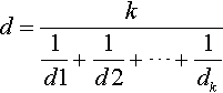
where di, 1 ≤ i ≤ k are the Euclidean distances between the solution whose harmonic distance is being calculated and each of its k-nearest neighbor solutions. The solutions with the largest harmonic distances are considered to be in the least crowded region of the objective space, and thus selected as survivors (lines 14 to 16).
Those familiar with MOEAs will note that HaD-MOEA is very similar to the well-known NSGA-II. HaD-MOEA was proposed with the aim of improving upon NSGA-II, which is known not to perform well when the number of objectives increases [209]. Wang et al. [438] explained that two key problems in NSGA-II are its measure of crowding distance and the method for selecting survivors based on it. NSGA-II uses the 1-norm distance between the two nearest neighbors of a solution as the crowding distance measure of this solution. Wang et al. [438] showed that this inherently does not reflect well the actual crowding degree of a given solution. In addition, NSGA-II calculates the crowding distance of a given solution based only on the solutions belonging to the same nondominated front as this solution. This obviously does not reflect the crowding distance considering all solutions selected so far, which is the real crowding of the solutions. So, in HaD-MOEA, the crowding distance is calculated based on both the solutions belonging to the same front and all the previously selected solutions. HaD-MOEA has been demonstrated to perform better than NSGA-II in the domain of optimal testing resource allocation when using three objectives [438].
Wang et al. [438] do not restrict HaD-MOEA to a specific parents selection mechanism. However, they use binary tournament selection in their experiments. As explained in Section 24.2, binary tournament selection works by picking two candidate solutions uniformly at random, and then selecting the best between them. A similar mechanism to the one used for survivor selection can be used to determine which of the two randomly picked candidate solutions is the “best.” This is repeated until the desired number of parents is obtained. The number of parents selected in this step depends on how the variation operators work, so as to generate the desired number of offspring. For example, if α offspring are to be generated and the crossover of two parents generates two offspring, then α parents must be selected. Note that, as crossover is probabilistic, there is some chance that it is not applied. In this case, the two parents could be cloned to produce two offspring. After crossover (or cloning), each offspring also has some chance to go through mutation.
24.4 Using MOEAs for creating see models
As explained by Harman and Clark [163], “[m]etrics, whether collected statically or dynamically, and whether constructed from source code, systems or processes, are largely regarded as a means of evaluating some property of interest.” For example, functional size and software effort are metrics derived from the project data. Performance measures such as MMRE, PRED, and LSD are metrics that represent how well a certain model fits the project data, and are calculated based on metrics such as software effort.
Harman and Clark [163] explain that metrics can be used as fitness functions in search-based software engineering, being able to guide the force behind the search for optimal or near optimal solutions in such a way to automate software engineering tasks. In that sense, search-based software engineering is very related to the construction of prediction models [162]. For instance, in the context of software cost/effort estimation, genetic programming has been applied using MSE as fitness function [102, 103, 386]. SEE was then innovatively proposed to be viewed as a multiobjective learning problem where the performance measures that we are interested in can be seen as separate objectives to be optimized by a MOEA in [319, 327], and soon after in [128, 376, 377].
This section explains the problem formulation and approach proposed by Minku and Yao [319, 327] to use MOEAs for creating SEE models. Different performance measures are used as objectives to be optimized simultaneously for generating SEE models. Different from single-objective formulations, that allows us to get a better understanding of different performance measures, to create well performing SEE ensembles, and to emphasize different performance measures if desired, as explained later in Section 24.5.
Once a representation, variation operators, and objective functions are defined, this approach can be used in combination with any MOEA. This chapter does not intend to show that a particular MOEA performs better or worse than another. For that reason, the evaluation of which MOEA is better for evolving SEE models is left as future work. In the current study, we concentrate on the multiobjective formulation of the problem, how to use a multiobjective approach to solve it, and providing a better understanding of different performance measures. Section 24.4.1 explains how we formulate the problem of creating SEE models as a multiobjective optimization problem, defining its objective functions. Section 24.4.2 comments on the type of SEE models generated. Section 24.4.3 explains the representation of the models and the variation operators used. Section 24.4.4 explains how to use the solutions produced by the MOEA.
24.4.1 Multiobjective formulation of the problem
Different performance measures can be used as objectives to be optimized when creating SEE models. In this work, considering a set of T projects, the following measures were used:
• Mean magnitude of the relative error:

where ![]() ;
; ![]() is the predicted effort; and yi is the actual effort.
is the predicted effort; and yi is the actual effort.
• Percentage of estimations within 25% of the actual values:

• Logarithmic standard deviation:

where s2 is an estimator of the variance of the residual ei and ![]() .
.
MMRE and LSD are objectives to be minimized, whereas PRED(25) is to be maximized. In order to avoid possible infinite LSD averages due to negative estimations, any negative estimation was replaced by the value one when calculating ![]() . MMRE and PRED(25) are popular metrics in the SEE literature, as illustrated by Table 2 of Dejaeger et al.'s [94] work, whereas LSD was recommended by Foss et al. [133] as being more reliable, especially for multiplicative models. These measures were chosen because, even though all of them were initially designed to represent how well a model performs, they are believed to behave very differently from each other, as confirmed in Section 24.6. This is potentially very useful for maximizing diversity among ensemble members, as explained in Chapter 20. Other measures can be investigated as future work.
. MMRE and PRED(25) are popular metrics in the SEE literature, as illustrated by Table 2 of Dejaeger et al.'s [94] work, whereas LSD was recommended by Foss et al. [133] as being more reliable, especially for multiplicative models. These measures were chosen because, even though all of them were initially designed to represent how well a model performs, they are believed to behave very differently from each other, as confirmed in Section 24.6. This is potentially very useful for maximizing diversity among ensemble members, as explained in Chapter 20. Other measures can be investigated as future work.
During the MOEA evolving procedure, the objective values are calculated using a set of projects with known effort, which will be referred to as the training set. When evaluating the results of the approaches, the performance measures are calculated over the test set.
Several different performance measures for SEE can be found in the literature. Most of them are calculated over the prediction error ![]() [297]. The mean absolute error (MAE) is the mean of the absolute prediction error, providing an unbiased measure that does not favor under- or overestimates. Sometimes median measures are used to avoid influence of extreme values. For these reasons, the evaluation analysis of our approach also considers its MAE, median absolute error (MdAE) and median MRE (MdMRE), which are defined as follows:
[297]. The mean absolute error (MAE) is the mean of the absolute prediction error, providing an unbiased measure that does not favor under- or overestimates. Sometimes median measures are used to avoid influence of extreme values. For these reasons, the evaluation analysis of our approach also considers its MAE, median absolute error (MdAE) and median MRE (MdMRE), which are defined as follows:
• ![]() ; and
; and
• MdMRE = Median {MREi/1 ≤ i ≤ T}.
24.4.2 See models generated
The models generated by the MOEA in this work are MLPs [32]. As explained in Section 24.1, MLPs can improve over conventional linear models when the function being modeled is not linear [422]. Even though we evolve MLPs in this work, MOEAs could also be used to generate other types of models for SEE, such as RBFs, RTs and linear regression equations. As the key point of this work is to analyze the multiobjective formulation of the creation of SEE models, and not the comparison among different types of models, the experimentation of MOEAs to create other types of models is left as future work.
24.4.3 Representation and variation operators
The MLP models were represented by a real value vector of size ni · (nh + 1) + nh · (no + 1), where ni, nh, and no are the number of inputs, hidden neurons, and output neurons, respectively. This real value vector is manipulated by the MOEA to generate SEE models. Each position of the vector represents a weight or the threshold of a neuron. The value one summed to nh and no in the formula above represents the threshold. The number of input neurons corresponds to the number of project input features and the number of output neurons is always one for the SEE task. The number of hidden neurons is a parameter of the approach.
The variation operators were inspired by Chandra and Yao's [69] work, which also involves evolution of MLPs. Let ![]() ,
, ![]() , and
, and ![]() be three parents. One offspring wc is generated with probability pc according to the following equation:
be three parents. One offspring wc is generated with probability pc according to the following equation:
where w is the real value vector representing the candidate solutions and N(0, σ2) is a random number drawn from a Gaussian distribution with mean zero and variance σ2.
An adaptive procedure inspired by simulated annealing is used to update the variance σ2 of the Gaussian at every generation [69]. This procedure allows the crossover to be initially explorative and then become more exploitative. The variance is updated according to the following equation:

where anneal_time is a parameter meaning the number of generations for which the search is to be explorative, after which σ2 decreases exponentially until reaching and keeping the value of one.
Mutation is performed elementwise with probability pm according to the following equation:
where wi represents a position of the vector representing the MLP and N(0, 0.1) is a random number drawn from a Gaussian distribution with mean zero and variance 0.1.
The offspring candidate solutions receive further local training using backpropagation [32], as in Chandra and Yao's [69] work.
24.4.4 Using the solutions produced by a MOEA
The solutions produced by the MOEA are innovatively used for SEE in two ways in this work. The first one is a Pareto ensemble composed of the best fit Pareto solutions. Best fit Pareto solutions are the Pareto solutions with the best train performance considering each objective separately. So, the ensemble will be composed of the Pareto solution with the best train LSD, best train MMRE, and best train PRED(25). The effort estimation given by the ensemble is the arithmetic average of the estimations given by each of its base models. So, each performance measure can be seen as having “one vote,” providing a fair and ideal trade-off among the measures when no emphasis is given to a certain measure over the others. This avoids the need for a software manager to decide on a certain measure to be emphasized.
It is worth noting that this approach to create ensembles focuses not only on accuracy, but also on diversity among base learners, which is known to be a key issue when creating ensembles [61, 244]. Accuracy is encouraged by using a MOEA to optimize MMRE, PRED, and LSD simultaneously. So, the base models are created in such a way to be generally accurate considering these three measures at the same time. Diversity is encouraged by selecting only the best fit Pareto solution according to each of these measures. As shown in Section 24.6, these measures behave very differently from each other. So, it is likely that the MMRE of the best fit Pareto solution according to LSD will be different from the MMRE of the best fit Pareto solution according to MMRE itself. The same is valid for the other performance measures. Models with different performance considering a particular measure are likely to produce different estimations, being diverse.
The second way to use the solutions produced by the MOEA is to use each best fit Pareto solution by itself. These solutions can be used when a particular measure is to be emphasized.
It is worth noting that a MOEA automatically creates these models. The Pareto solutions and the best fit Pareto solutions can be automatically determined by the algorithm. There is no need to invole manual/visual checking.
24.5 Experimental setup
The experiments presented in this chapter were designed to answer research questions RQ1-RQ3 explained in the beginning of the chapter. In our experiments, HaD-MOEA (Section 24.3) has been used as the MOEA algorithm for generating MLP SEE models, due to its simplicity and advantages over NSGA-II (see Section 24.3). Our implementation of HaD-MOEA was based on the meta-heuristic optimization framework for Java Opt4J [273]. MLP SEE models were generated according to Section 24.4.
In order to answer RQ1, we show that plots of the Pareto solutions can be used to provide a better understanding of the relationship among different performance measures. They can show that, for example, when increasing the value of a certain measure, the value of another measure may decrease and by how much. Our study shows the very different and sometimes even opposite behavior of different measures. This is an indicator that these measures can be used to create diverse ensembles for SEE (Section 24.6).
In order to answer RQ2, the following comparison was made (Section 24.7):
• Pareto ensemble versus backpropagation MLP (single MLP created using backpropagation). This comparison was made to show the applicability of MOEAs to generate SEE ensemble models. It analyzes the use of a MOEA, which considers several performance measures at the same time, against the nonuse of a MOEA.
The results of this comparison show that the MOEA is successful in generating SEE ensemble models by optimizing different performance measures explicitly at the same time. These ensembles present performance similar to or better than a model that does not optimize the three measures concurrently. Furthermore, the similar or better performance is achieved considering all the measures used to create the ensemble, showing that these ensembles not only provide a better trade-off among different measures, but also improve the performance considering these measures.
In order to answer RQ3, the following comparison was made (Section 24.8):
• Best fit Pareto MLP versus Pareto ensemble. This comparison allows us to check whether it is possible to increase the performance considering a particular measure if we would like to emphasize it. This is particularly useful when there is a certain measure that we believe to be more appropriate than the others.
The results of this comparison reveal that MOEAs are flexible in terms of providing SEE models based on a multiobjective formulation of the problem. They can provide both solutions considered as having a good trade-off when no measure is to be emphasized and solutions that emphasize certain measures over the others if desired. If there is no measure to be emphasized, a Pareto ensemble can be used to provide a relatively good performance in terms of different measures. If the software manager would like to emphasize a certain measure, it is possible to use the best fit Pareto solution in terms of this measure.
Additionally, the following comparisons were made to test the optimality of the choice of best fit MLPs as models to be used (Section 24.9):
• Best Pareto MLP in terms of test performance versus backpropagation MLP, and Pareto ensemble composed of the best Pareto MLPs in terms of each test performance versus backpropagation MLP. This comparison was made to check whether better results could be achieved if a better choice of solution from the Pareto front was made. Please note that choosing the best models based on their test performance was done for analysis purposes only and could not be done in practice.
The results of this comparison show that there is still room for improvement in terms of Pareto solution choice.
The comparisons to answer the research questions as outlined above show that it is possible and worth considering SEE models generation as a multiobjective learning problem and that a MOEA can be used to provide a better understanding of different performance measures, to create well-performing SEE ensembles, and to create SEE models that emphasize particular performance measures.
In order to show how the solutions generated by the HaD-MOEA to evolve MLPs compare to other approaches in the literature, an additional round of comparisons was made against the following methods (Section 24.10):
• Single learners: MLPs [32]; RBFs [32]; RTs [459]; and estimation by analogy (EBA) [390] based on log transformed data.
• Ensemble learners: bagging [46] with MLPs, with RBFs and with RTs; random [156] with MLPs; and negative correlation learning (NCL) [263, 264] with MLPs.
These comparisons do not evaluate the multiobjective formulation of the problem by itself, but a mix of the HaD-MOEA to the type of models being evolved (MLP). According to very recent studies [223, 321, 326], REPTrees, bagging ensembles of MLPs, bagging ensembles of REPTrees, and EBA based on log transformed data can be considered to be among the best current methods for SEE. The implementation used for all the opponent learning machines but NCL was based on Weka [156]. The RTs were based on the REPTree model. We recommend the software Weka should the reader wish to get more details about the implementation and parameters. The software used for NCL is available upon request.
The results of these comparisons show that the MOEA-evolved MLPs were ranked first more often in terms of MMRE, PRED(25), MdMRE, MAE, and MdAE, but performed less well in terms of LSD. They were also ranked first more often for the International Software Benchmarking Standards Group (ISBSG) (cross-company) data sets, which are likely to be more heterogeneous. It is important to emphasize, though, that this additional comparison is not only evaluating the MOEA and the multiobjective formulation of the problem, but also the type of model being evolved (MLP). Other types of models could also be evolved by the MOEA and could possibly provide better results in terms of LSD.
The experiments were based on the PROMISE data sets explained in Section 20.4.1.1, the ISBSG subsets explained in Section 20.4.1.2, and a data set containing the union of all the ISBSG subsets (orgAll). The union was used in order to create a data set likely to be more heterogeneous than the previous ones.
Thirty rounds of executions were performed for each data set from Section 20.4.1. In each round, for each data set, 10 projects were randomly picked for testing and the remaining were used for the MOEA optimization process/training of approaches. Holdout of size 10 was suggested by Menzies et al. [292] and allows the largest possible number of projects to be used for training without hindering the testing. For the data set sdr (described in Section 20.4.1.1), half of the projects were used for testing and half for training, due to the small size of the data set. The measures of performance used to evaluate the approaches are MMRE, PRED(25), and LSD, which are the same performance measures used to create the models (Section 24.4.1), but calculated on the test set. It is worth noting that MMRE and PRED using the parameter 25 were chosen for being popular measures, even though raw values from different papers are not directly comparable because they use different training and test sets, besides possibly using different evaluation methods. In addition, we also report MdMRE, MAE, and MdAE.
The absolute value of the Glass's Δ effect size [373] was used to evaluate the practical significance of the changes in performance when choosing between the Pareto ensemble and an opponent approach:
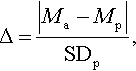
where Mp and Ma are the performances obtained by the Pareto ensemble and an opponent approach, and SDp is the standard deviation obtained by the Pareto ensemble. As the effect size is scale-free, it was interpreted based on Cohen's [80] suggested categories: small (≈ 0.2), medium (≈ 0.5), and large (≈ 0.8). Medium and large effect sizes are of more “practical” significance.
The parameters choice of the opponent approaches was based on five preliminary executions using several different parameters (Table 24.1). The set of parameters leading to the best MMRE for each data set was used for the final 30 executions used in the analysis. MMRE was chosen for being a popular measure in the literature. The experiments with the opponent approaches were also used by Minku and Yao [321].
Table 24.1
Parameter Values for Preliminary Executions

Note: From [327].
The MLP's learning rate, momentum, and number of hidden neurons used by HaD-MOEA were chosen so as to correspond to the parameters used by the opponent backpropagation MLPs and are presented in Table 24.2. These parameters were tuned to provide very good results for the opponent backpropagation MLPs, but were not specifically tuned for the MOEA approach described in this chapter. The number of generations, also shown in Table 24.2, is the number of epochs used by the opponent backpropagation MLPs divided by the number of epochs for the offspring backpropagation. This value was chosen so that each MLP at the end of the evolutionary process is potentially trained with the same total number of epochs as the opponent backpropagation MLPs. The remaining evolutionary parameters were fixed for all data sets and were not intended to be optimal. In summary, these are
Table 24.2
Parameter Values Used in the HaD-MOEA
| Data Set | Learning Rate | Momentum | # Generations | # Hidden Neurons |
| Cocomo81 | 0.3 | 0.5 | 200 | 9 |
| Sdr | 0.5 | 0.2 | 20 | 9 |
| Nasa | 0.1 | 0.1 | 100 | 9 |
| Desharnais | 0.1 | 0.1 | 100 | 9 |
| Nasa93 | 0.4 | 0.5 | 20 | 5 |
| Org1 | 0.1 | 0.2 | 200 | 9 |
| Org2 | 0.1 | 0.1 | 100 | 5 |
| Org3 | 0.1 | 0.3 | 100 | 5 |
| Org4 | 0.2 | 0.3 | 200 | 9 |
| Org5 | 0.2 | 0.3 | 200 | 9 |
| Org6 | 0.1 | 0.1 | 20 | 3 |
| Org7 | 0.5 | 0.3 | 20 | 5 |
| OrgAll | 0.1 | 0.5 | 20 | 9 |
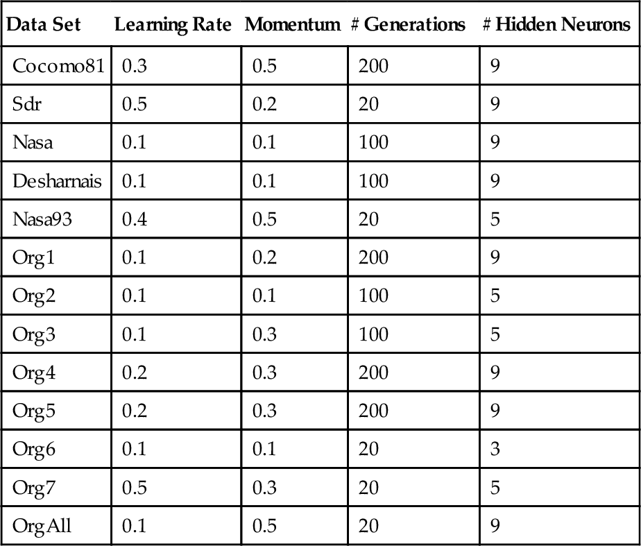
Note: From [327].
• Tournament size: 2 (binary tournament selection). Tournament is a popular parent selection method. A tournament size of 2 is commonly used in practice because it often provides sufficient selection pressure on the most fit candidate solutions [248].
• Population size: 100. This value was arbitrarily chosen.
• Number of epochs used for the backpropagation applied to the offspring candidate solutions: 5. This is the same value as used by Chandra and Yao [69].
• Anneal_time: number of generations divided by 4, as in Chandra and Yao's [69] work.
• Probability of crossover: 0.8. Chosen between 0.8 and 0.9 (the value used by Wang et al. [438]) so as to reduce the MMRE in five preliminary executions for cocomo81. We decided to check whether 0.8 would be better than 0.9 because 0.9 can be considered as a fairly large probability.
• Probability of mutation: 0.05. Chosen between 0.05 and 0.1 (the value used by Wang et al. [438]) so as to reduce the MMRE in five preliminary executions for cocomo81. We decided to check whether 0.05 would be better than 0.1 because the value 0.1 can be considered large considering the size of each candidate solution of the population in our case.
A population size arbitrarily reduced to 30 and number of epochs for the offspring backpropagation reduced to zero (no backpropagation) were used for additional MOEA executions in the analysis. Unless stated otherwise, the original parameters summarized above were used.
The analysis presented in this chapter is based on five data sets from the PRedictOr Models In Software Engineering Software (PROMISE) Repository [300] and eight data sets based on the ISBSG Repository [271] Release 10, as in [321]. The data sets were the same as the ones used in Chapter 20 (cocomo81, nasa93, nasa, sdr, desharnais, org1-org7 and orgAll) and chosen to cover a wide range of problem features, such as number of projects, types of features, countries and companies.
24.6 The relationship among different performance measures
This section presents an analysis of the Pareto solutions with the aim of providing a better understanding of the relationship among MMRE, PRED(25), and LSD (RQ1). All the plots presented here refer to the execution among the 30 runs in which the Pareto ensemble obtained the median test MMRE, unless its test PRED(25) was zero. In that case, the nonzero test PRED(25) execution closest to the median MMRE solution was chosen. This execution will be called median MMRE run.
Figure 24.5 presents an example of Pareto solutions plot for nasa93. We can see that solutions with better PRED(25) do not necessarily have better MMRE and LSD. The same is valid for the other performance measures. For example, a solution with relatively good MMRE may have very bad LSD, and a solution with good LSD may have very bad PRED(25). This demonstrates that model choice or creation based solely on one performance measure may not be ideal. In the same way, choosing a model based solely on MMRE when the difference in MMRE is statistically significant [292] may not be ideal.

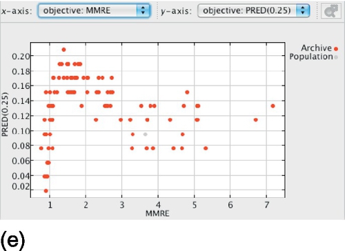
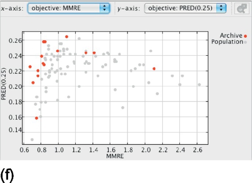
In order to better understand the relationship among the performance measures, we plotted graphs LSD versus MMRE, LSD versus PRED(25), and MMRE versus PRED(25) for the median MMRE run, for each PROMISE data set and for ISBSG orgAll. Figure 24.6 shows representative plots for cocomo81 and orgAll. Other figures were omitted due to space restrictions and present the same tendencies. It is worth noting that, even though some Pareto solutions have worse performance than other solutions considering the two measures in the plots, they are still nondominated when all three objectives are considered. All the three objectives have to be considered at the same time to determine whether a solution is (non)dominated.
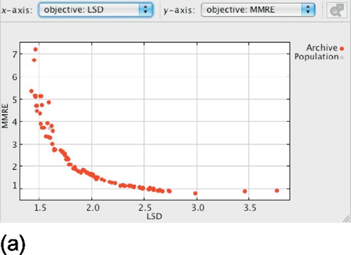


Considering LSD versus MMRE (Figure 24.6a and b), we can see that as MMRE is improved (reduced), LSD tends to get worse (increased). This tendency is particularly noticeable for cocomo81, which contains more solutions in the Pareto front.
Considering LSD versus PRED(25) (Figure 24.6c and d), we can see that solutions with similar PRED(25) frequently present different LSD. The opposite is also valid: solutions with similar LSD frequently present different PRED(25). As PRED(25) is the percentage of estimations within 25% of the actual effort, one would expect several solutions with different LSD to have the same PRED(25), as a big improvement is necessary to cause impact on PRED(25). The opposite is somewhat more surprising. It indicates that average LSD by itself is not necessarily a good performance measure and may be affected by a few estimations containing extreme values.
A similar behavior is observed in the graphs MMRE versus PRED(25) (Figure 24.6e and f), but it is even more extreme in this case: Solutions with even more different MMRE present the same PRED(25).
Overall, the plots show that, even though a certain solution may appear better than another in terms of a certain measure, it may be actually worse in terms of the other measures. As none of the existing performance measures has a perfect behavior, the software manager may opt to analyze solutions using several different measures, instead of basing decisions on a single measure. For instance, s/he may opt for a solution that behaves better considering most performance measures. The analysis also shows that MMRE, PRED(25), and LSD behave differently, indicating that they may be useful for creating SEE ensembles. This is further investigated in Section 24.7.
Moreover, considering this difference in behavior, the choice of a solution by a software manager may not be easy. If the software manager has a reason for emphasizing a certain performance measure, s/he may choose the solution more likely to perform best for this measure. However, if it is not known what measure to emphasize, s/he may be interested in a solution that provides a good trade-off among different measures. We show in Section 24.7 that MOEA can be used to automatically generate an ensemble that provides a good trade-off among different measures, so that the software manager does not necessarily need to decide on a particular solution or performance measure. Our approach is also robust, allowing the software manager to emphasize a certain measure should s/he wish to, as shown in Section 24.8.
24.7 Ensembles based on concurrent optimization of performance measures
This section concentrates on answering RQ2. As explained in Section 24.6, different measures behave differently, indicating they may provide a natural way to generate diverse models to compose SEE ensembles. In this section, we show that the best fit MOEA Pareto solutions in terms of each objective can be combined to produce an SEE ensemble (Pareto ensemble) that achieves good results in comparison to a traditional algorithm that does not consider several different measures explicitly. So, the main objective of the comparison presented in this section is to analyze whether MOEA can be used improve the performance over the nonuse of MOEA considering the same type of base models. Comparison with other types of models is shown in Section 24.10.
The analysis is done by comparing the Pareto ensemble of MLPs created by the MOEA as explained in Section 24.4 to MLPs trained using backpropagation [32], which is the learning algorithm most widely used for training MLPs. Each best fit solution used to create the Pareto ensemble is the one with the best train performance considering a particular measure. The Pareto ensemble represents a good trade-off among different performance measures, if the software manager does not wish to emphasize any particular measure.
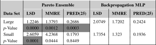
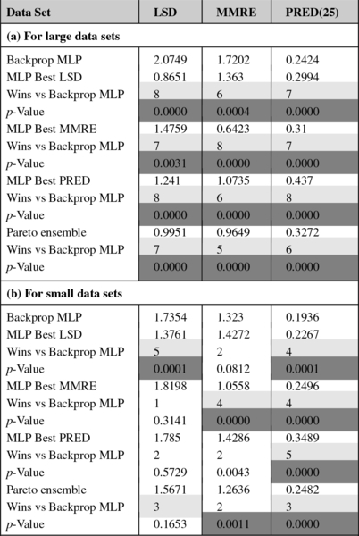
First, let's analyze the test performance average considering all data sets. Table 24.3 shows the average test performance and standard deviation for the Pareto ensemble and the backpropagation MLP. The cells in light gray represent better averages (not necessarily statistically different). The table also shows the overall average and p-value of the Wilcoxon test used for the statistical comparison of all runs over multiple data sets. p-Values less than 0.0167 (shown in dark gray) indicate statistically significant difference using Bonferroni corrections considering the three performance measures at the overall level of significance of 0.05. As we can see, the two approaches are statistically the same considering the overall MMRE, but different when considering LSD and PRED(25). In the latter case, the Pareto ensemble wins in 7 out of 13 data sets considering LSD and PRED(25), as shown by the light gray cells. This number of wins is similar to the number of losses, so additional analysis is necessary to better understand the Pareto ensemble's behavior and check if it can be improved, as shown in the next paragraphs.
Table 24.3
Pareto Ensemble vs Backpropagation MLP—Test Performance Average and Standard Deviation
 |

From [327].
Notes: The p-values of the Wilcoxon tests for the comparison over multiple data sets are also shown. p-Values less than 0.0167 indicate statistically significant difference using Bonferroni corrections at the overall level of significance of 0.05 and are in dark gray. The cells in light gray represent better averages (not necessarily statistically different).
Hence, second, if we take a closer look, we can see that backpropagation MLP frequently wins for the smallest data sets, whereas the Pareto ensemble tends to behave better for the largest data sets. Considering LSD, the Pareto ensemble wins in 6 out of 8 large data sets. Considering MMRE, it wins in 5 out of 8 large data sets. Considering PRED(25), it wins in 7 out of 8 large data sets. So, we performed additional statistical tests to compare the behavior of all the runs considering the data sets with less than 35 projects (sdr, org2, org5, org6, org7) and with 60 or more projects (cocomo81, nasa93, nasa, desharnais, org1, org3, org4, orgAll) separately.
Table 24.4 shows the overall averages and p-values for these two groups of data sets. We can see that there is statistically significant difference considering all performance measures for the large data sets, including MMRE. That, together with the fact that the Pareto ensemble wins in most cases for these data sets, indicates that it is likely to perform better than backpropagation MLPs for large data sets. That is a very good achievement, especially considering that the backpropagation MLPs were very well tuned for providing good MMRE. For the small data sets, the two approaches obtained were statistically significantly different LSD and the Pareto ensemble was worse in 4 out of 5 small data sets. The two approaches were statistically equal in terms of MMRE and PRED(25) for the small data sets.
Table 24.4
Pareto Ensemble vs Backpropagation MLP Considering Large and Small Data Sets Separately—Test Performance
 |

From [327].
Notes: The p-values of the Wilcoxon tests for the comparison over multiple data sets are also shown. p-Values less than 0.0167 indicate statistically significant difference using Bonferroni corrections at the overall level of significance of 0.05 and are in dark gray.
A possible reason for the worse behavior for the smallest data sets is overfitting. To make this hypothesis more well-grounded, we checked the MMREs obtained by each MLP of the Pareto ensemble for the median MMRE run of org5. Org5 was chosen for being the data set in which the Pareto ensemble obtained the worst test MMRE, but not the one with the smallest number of projects, as only 12 projects may be too little for a significant analysis. The test MMREs were 1.9396, 1.9217, and 1.9613, whereas the corresponding train MMREs were 0.0998, 0.0976, and 0.1017, respectively. We can see that the test MMREs were drastically larger than the train MMREs. On the other hand, the three runs on and around the median test MMRE for the backpropagation MLPs obtained 1.0403, 1.0433, and 1.1599 test MMRE, whereas the train MMREs were 0.3183, 1.0857, and 0.1176. So, the train MMREs were higher (worse) for the backpropagation MLPs than for the best fit Pareto MLPs. That indicates that the MOEA may indeed be overfitting when the data sets are too small. Besides the fact that learning is inherently hard due to the small number of training examples, a possible cause for that is the parameters choice, as the parameters were not so well-tuned for the MOEA.
So, third, additional MOEA runs were performed in such a way to use the essence of the early stopping strategy to avoid overfitting [131]. This was done by reducing the population size from 100 to 30 and the number of epochs for the offspring backpropagation from 5 to 0 (no backpropagation). The results are shown in Table 24.5. As we can see, the Pareto ensemble obtained similar LSD and MMRE to backpropagation MLPs. PRED(25) was statistically significantly different and the Pareto ensemble won in 3 out of 5 data sets. The improvement in the overall average was of about 0.79 for LSD, 2.44 for MMRE, and 0.04 for PRED(25). The test MMREs for the median MMRE run of the Pareto ensemble for org5 were 0.8649, 0.8528, and 1.4543, whereas the corresponding train MMREs were 0.3311, 0.3116, and 0.5427. These train MMREs are closer to the corresponding test MMREs than when using the previous parameters configuration, indicating less overfitting.
Table 24.5
Pareto Ensemble Using Adjusted Parameters (Reduced Population Size and No Backpropagation) vs Backpropagation MLP for Small Data Sets—Test Performance and Standard Deviation
 |

From [327].
Notes: The p-values of the Wilcoxon tests for the comparison over multiple data sets are also shown. p-Values less than 0.0167 indicate statistically significant difference using Bonferroni corrections at the overall level of significance of 0.05 and are in dark gray. The cells in light gray represent better averages (not necessarily statistically different).
Last, in order to check the performance of the Pareto ensemble for outlier projects, we have also tested it using test sets comprised only of the outliers identified in Section 20.4.1. The MMRE and PRED(25) obtained for the outlier sets were compared to the original test sets. It is not possible to compare LSD because the number of outliers is too small and LSD's equation is divided by the number of projects minus one. So, even if the error obtained for the outlier sets is potentially smaller, the small number of examples increases LSD.
The results show that PRED(25) was always worse for the outlier sets than for the original test sets. That means that these outliers are projects to which the Pareto ensemble has difficulties in predicting within 25% of the actual effort. However, the MMRE is actually better for 3 out of 9 data sets that involve outliers. So, in about a third of the cases, the outliers are not projects to which the Pareto ensemble obtains the worst performances. For the other cases, the MMRE was usually less than 0.27 higher.
The analysis performed in this section shows that the use of MOEA for considering several performance measures at the same time is successful in generating SEE ensembles. The Pareto ensemble manages to obtain similar or better performance than backpropagation MLP across data sets in terms of all the measures used as objectives by the MOEA. So, it is worth considering the creation of SEE models as a multiobjective problem and the Pareto ensemble can be used when none of the performance measures is to be emphasized over the others.
24.8 Emphasizing particular performance measures
This section concentrates on answering RQ3. As shown in Section 24.7, MOEA can be used to automatically generate an ensemble that provides an ideal trade-off among different measures, so that the software manager does not need to decide on a particular solution or performance measure. The main objective of the comparison presented in the present section is to analyze whether we can further increase the test performance for each measure separately if we wish to emphasize this particular measure. This section provides a better understanding of the solutions that can be produced by the MOEA and shows that our approach is robust in the case where the manager wishes to emphasize a certain measure. In order to do so, we check the performance of the best fit solution considering each objective separately. The best fit solution is the one with the best train performance considering a particular measure.
Table 24.6a and b shows the results of the comparisons between the best fit Pareto MLP in terms of each objective versus the Pareto ensemble for large and small data sets, respectively. The MOEA parameters for the small data sets are the ones with population size 30 and no backpropagation. Dark gray color means statistically significant difference using Wilcoxon tests with Bonferroni corrections at the overall level of significance of 0.05 (statistically significant difference when p-value < 0.05/(3 * 3)). The number of times in which each approach wins against the Pareto ensemble is also shown and is in light gray when the approach wins more times.
Table 24.6
Test Performance Average of Best Fit Pareto MLPs Against the Pareto Ensemble
 |

From [327].
Notes: The adjusted MOEA parameters were used for the small data sets. The p-values of the Wilcoxon tests for the comparison over multiple data sets are also shown. p-Values less than 0.0056 (in dark gray) indicate statistically significant difference using Bonferroni corrections at the overall level of significance of 0.05. When the best fit Pareto MLP wins more times than the Pareto ensemble, its number of wins is highlighted in light gray.
The results of these comparisons indicate that using each best fit Pareto MLP considering a certain objective can sometimes improve the test performance considering this objective. Even though the test performance to be emphasized becomes equal or better than the Pareto ensemble, as shown by the statistical test and the number of wins, the performance considering the other measures gets equal or worse. It is worth noting, though, that the best fit Pareto MLPs are still nondominated solutions, providing acceptable performance in terms of all the measures in comparison to other solutions generated by the MOEA.
In addition to the statistical comparison, we are also interested in the effect size Δ (Equation (24.1), Section 24.5) of each best MLP in comparison to the Pareto ensemble, in terms of the performance measure for which the MLP performs best. Table 24.7 presents the minimum, maximum, average, and standard deviation of the effect size Δ, as well as the number of data sets for which the effect size was small, medium, or large. Even though using each best MLP separately can provide some improvement in performance, the improvements are usually small. Nevertheless, as it would be very easy to configure an approach to use the best MLPs instead of the Pareto ensemble, one may wish to use the best MLPs to emphasize a certain performance measure even considering that the improvement in performance is small.
Table 24.7
Effect Size for Each Best MLP Against the Pareto Ensemble, in Terms of the Performance Measure for Which the MLP Performs Best
| Min. Δ | Max. Δ | Avg. Δ | Std Δ | # Small | # Medium | # Large | # Medium + Large | |
| (a) Large data sets | ||||||||
| Best LSD MLP | 0.0257 | 0.3221 | 0.1395 | 0.0993 | 8 | 0 | 0 | 0 |
| Best MMRE MLP | 0.0046 | 0.7983 | 0.3462 | 0.3035 | 4 | 3 | 1 | 4 |
| Best PRED MLP | 0.0542 | 0.2953 | 0.1699 | 0.0987 | 8 | 0 | 0 | 0 |
| (b) Small data sets | ||||||||
| Best LSD MLP | 0.0294 | 0.4468 | 0.2009 | 0.1687 | 4 | 1 | 0 | 1 |
| Best MMRE MLP | 0.0567 | 0.5913 | 0.2665 | 0.2080 | 4 | 1 | 0 | 1 |
| Best PRED MLP | 0.0235 | 0.9502 | 0.4050 | 0.3977 | 2 | 1 | 2 | 3 |

Note: From [327].
24.9 Further analysis of the model choice
The main objective of the comparison presented in this section is to analyze whether our approach still has room for improvement in terms of model choice. If so, as future work, other methods for choosing models for the Pareto ensemble should be investigated with the aim of improving this approach further. In order to make this analysis, we used the best Pareto MLPs according to each test performance. These MLPs represent the best possible choice of solutions generated by the MOEA considering each objective separately. A Pareto ensemble comprised of these MLPs was also formed. Table 24.8a and b shows the results of the comparisons for large and small data sets, respectively. Again, the parameters used by the MOEA for the small data sets here are the ones with population size 30 and no backpropagation. Wilcoxon tests with Bonferroni corrections at the overall significance level of 0.05 (statistically significant difference when p-value < 0.05/(3 * 4)) were used to aid the comparison.
Table 24.8
Test Performance Average of Best Test Performing Pareto MLPs Against Backpropagation MLP
 |

From [327].
Notes: The adjusted MOEA parameters were used for the small data sets. The p-values of the Wilcoxon tests for the comparison over multiple data sets are also shown. p-Values less than 0.0042 (in dark gray) indicate statistically significant difference using Bonferroni corrections at the overall level of significance of 0.05. When the best test performing Pareto MLP wins more times than the backpropagation MLP, its number of wins is highlighted in light gray.
We can see that there are test performance improvements in almost all cases, both when using the best Pareto MLPs by themselves and when combining them into a Pareto ensemble. In particular, for most results with statistically significant difference in the average LSD, MMRE, or PRED(25), the best test performance approach wins more times than the backpropagation MLPs. This analysis shows that, even though our approach can significantly reduce overfitting by reducing the population size and eliminating offspring backpropagation for smaller data sets, simply choosing the best fit Pareto MLPs according to the train performance still does not necessarily lead to the best achievable performance. As future work, other strategies to chose models among the Pareto solutions should be investigated to improve the performance even further.
24.10 Comparison against other types of models
The main objectives of RQ2 and RQ3 were to show that MOEAs can be used to evolve models considering different performance measures at the same time, being able to produce solutions that achieve good results in comparison to a traditional algorithm that does not use several different measures explicitly to generate the same type of models, besides being flexible to allow emphasizing different performance measures. The analyses explained in Sections 24.7, 24.8 answer RQ2 and RQ3. Nevertheless, even though it is not the key point of this work, it is still interesting to know how well HaD-MOEA to evolve MLPs behaves in comparison to other types of models. Differently from the previous analyses, this comparison mixes the evaluation of the MOEA to the evaluation of the underlying model being evolved (MLP).
In this section, we present a comparison of the Pareto ensemble to several different types of model besides MLPs: RBFs, RTs, EBA with log transformed data, bagging with MLPs, bagging with RBFs, bagging with RTs, random with MLPs, and NCL with MLPs, as explained in Section 24.5. For this comparison, the parameters used by the MOEA on the small data sets were adjusted to population size of 30 and no offspring backpropagation. The performance measures used to evaluate the models are LSD, MMRE, PRED(25), MdMRE, MAE, and MdAE.
The first step of our analysis consists of performing Friedman tests [96] for the statistical comparison of multiple models over multiple data sets for each performance measure. The null hypothesis is that all the models perform similarly according to the measure considered. The tests rejected the null hypothesis for the six performance measures with Holm-Bonferroni corrections at the overall level of significance of 0.05. The Friedman tests also provide rankings of the approaches across data sets, which show that Pareto ensemble, bagging + MLPs, log + EBA, and RTs have the top half average ranks considering all measures but LSD. Models based on MLPs, including the Pareto ensemble, tend to be lower ranked considering LSD. A closer analysis of the MLPs revealed that they can sometimes make negative estimations, which have a strong impact on LSD. RTs, on the other hand, can never give negative estimations or estimations close to zero when the training data does not contain such effort values. So, learners based on RTs obtained, in general, better LSD. Bagging + RTs was the highest ranked approach in terms of both LSD and MAE.
It is important to note that MOEAs could also be used to evolve other types of structure than MLPs. However, the key point of this work is the investigation of the multiobjective formulation of the problem of creating SEE models and obtaining a better understanding of the performance measures. The use of MOEA to evolve other types of models such as RTs, which could improve LSD, is proposed as future work.
It is also interesting to verify the standard deviation of the Friedman ranking across different performance measures. The Pareto ensemble and log + EBA presented the median standard deviation, meaning that their average ranking across data sets does not vary too much when considering different performance measures, even though they are not the approaches that vary the least. Bagging + MLPs presented the lowest and bagging + RTs presented the highest standard deviation.
Nevertheless, simply looking at the ranking provided by the Friedman test is not very descriptive for SEE, as the models tend to behave very differently depending on the data set. Ideally, we would like to use the approach that is most suitable for the data set in hand. So, as the second step of our analysis, we determine what approaches are ranked first according to the test performance on each data set separately. This is particularly interesting because it allows us to identify on what type of data sets a certain approach behaves better. Table 24.9 shows the approaches ranked as first considering each data set and performance measure. Table 24.10a helps us to see that the Pareto ensemble appears more often as the first than the other approaches in terms of all measures but LSD. Table 24.10b shows that the Pareto ensemble is never ranked last more than twice considering all 13 data sets and it is only ranked worse twice in terms of MMRE. For the reason explained in the previous paragraphs, approaches based on MLPs are rarely ranked first in terms of LSD, whereas bagging + RTs and RTs are the approaches that appear most often as first in terms of this measure.
Table 24.9
Approaches Ranked as First per Data Set
| Approach | LSD | MMRE | PRED(25) | MdMRE | MAE | MdAE |
| Cocomo81 | RT | Bag + MLP | Bag + MLP | Bag + MLP | Bag + MLP | Bag + MLP |
| Sdr | RT | RT | Bag + RT | RT | RT | RBF |
| Nasa | Bag + RT | RT | Bag + MLP | Bag + MLP | Bag + RT | Bag + RT |
| Desharnais | Bag + RT | Bag + MLP | Pareto Ens | Pareto Ens | Pareto Ens | Pareto Ens |
| Nasa93 | RT | RT | RT | RT | RT | RT |
| Org1 | Bag + RBF | Pareto Ens | Pareto Ens | Pareto Ens | Pareto Ens | Pareto Ens |
| Org2 | Bag + RT | Pareto Ens | Pareto Ens | Pareto Ens | Pareto Ens | Pareto Ens |
| Org3 | Pareto Ens | Pareto Ens | Log + EBA | Log + EBA | Log + EBA | Log + EBA |
| Org4 | Bag + RBF | Pareto Ens | RT | RT | Pareto Ens | Pareto Ens |
| Org5 | Bag + RT | Log + EBA | Bag + RBF | Rand + MLP | Bag + RT | RT |
| Org6 | Bag + RBF | Pareto Ens | Pareto Ens | Pareto Ens | Bag + RBF | Pareto Ens |
| Org7 | Bag + RT | Log + EBA | Log + EBA | Log + EBA | Bag + RBF | Pareto Ens |
| OrgAll | RT | Pareto Ens | Pareto Ens | Pareto Ens | Pareto Ens | Pareto Ens |

Note: From [327].
Table 24.10
Approaches Ranked as First—Summary
 |

From [327].
Note: Values higher than 3 are highlighted in gray.
Table 24.9 also reveals that the Pareto ensemble was first more often for the ISBSG data sets than for the PROMISE data sets. ISBSG data sets are considered as very heterogeneous. So, MOEAs might be particularly useful for more heterogeneous data. A possible reason for that is that the Pareto ensemble uses a global optimization algorithm, which is usually better at identifying the most promising regions of the search space than local algorithms such as backpropagation. More heterogeneous data sets may present search surfaces with several peaks, more difficult to tackle by local search algorithms.
As a third step of our analysis, the absolute value of the effect size Δ (Equation (24.1), Section 24.5) using MAE as the performance measure were calculated (Table 24.11). We report Δ based on MAE because this performance measure is symmetric/unbiased. As we can see, many of the effect sizes are medium or large. So, the choice of a certain approach instead of the Pareto ensemble can have a big impact on the performance of the SEEs.
Table 24.11
Effect Size for Each Approach Against the Pareto Ensemble
| Approach | Min. Δ | Max. Δ | Avg. Δ | Std Δ | # Small | # Medium | # Large | # Medium + Large |
| Bag + MLP | 0.0296 | 0.9194 | 0.3775 | 0.2839 | 7 | 4 | 2 | 6 |
| Bag + RBF | 0.0046 | 1.3072 | 0.5007 | 0.4233 | 6 | 3 | 4 | 7 |
| Bag + RT | 0.0518 | 1.3383 | 0.4842 | 0.4195 | 7 | 3 | 3 | 6 |
| Log + EBA | 0.0199 | 1.4054 | 0.5333 | 0.4839 | 7 | 2 | 4 | 6 |
| MLP | 0.0202 | 1.5049 | 0.4155 | 0.4034 | 7 | 3 | 3 | 6 |
| NCL | 0.0170 | 2.4236 | 0.7194 | 0.6534 | 5 | 3 | 5 | 8 |
| Rand | 0.0720 | 1.5655 | 0.4615 | 0.4444 | 7 | 3 | 3 | 6 |
| RBF | 0.0393 | 1.5730 | 0.6207 | 0.5299 | 6 | 2 | 5 | 7 |
| RT | 0.0392 | 1.8151 | 0.5614 | 0.5203 | 4 | 6 | 3 | 9 |
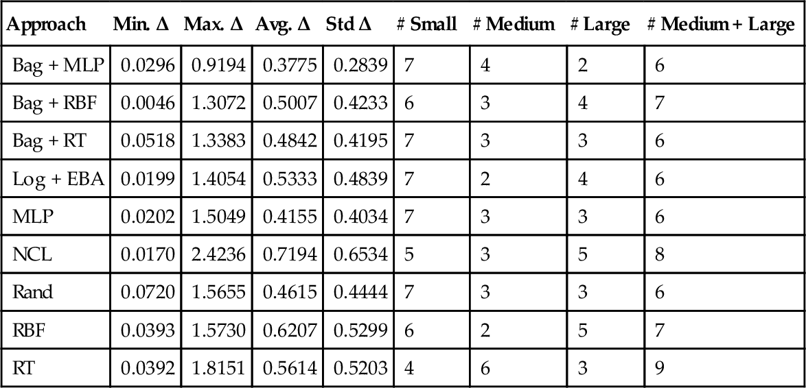
Note: From [327].
Finally, it is also worth noting that, in terms of computational time, some approaches such as log + EBA are faster than the MOEA. However, we do not consider the differences as of practical significance, because our approach did not present high running time. The reasons for the low running time are (1) SEE data sets are usually small in comparison to other ML applications and (2) our results were obtained without running the MOEA for too many generations. As an example, one run for the largest, the second largest, and the third largest data sets, which use 20, 100, and 200 generations, respectively, takes less than 1 minute to finish.
In summary, this section shows that MOEA-evolved MLPs are able to achieve competitive results in comparison to other approaches in the literature. The Pareto ensemble usually obtained comparatively good results in terms of all measures but LSD. Whether this is acceptable is problem (project) dependent and also depends on the magnitude of loss in terms of LSD compared to the gain in other measures. Moreover, the Pareto ensemble seems to perform better for more heterogeneous data sets such as ISBSG.
24.11 Summary
This chapter demonstrates how to view the problem of creating SEE models through a different perspective, by tackling it as a multiobjective problem that considers different performance measures explicitly and simultaneously. Using a MOEA to solve this problem allows us to better understand different performance measures and to produce SEE models with good overall performance in comparison to a model that does not consider these measures explicitly.
As an answer to RQ1, we show that LSD and MMRE are performance measures with somewhat opposite behavior. Moreover, models with similar LSD/MMRE are likely to present different PRED(25) and vice versa. So, one may wish to choose a model that does not behave particularly bad for any intended performance measures. This is one of the motivations for our approach to use MOEAs, as MOEAs consider all these performance measures at the same time. This difference in behavior also provides the second motivation for our approach: it can produce diverse ensembles, which are more likely to have increased performance.
The results above indicate that considering different performance measures explicitly when creating a model may be used to produce good ensembles. As an answer to RQ2, we show that indeed a MOEA can be used to create models by explicitly considering different performance measures at the same time. Pareto ensemble of MLPs produced by a MOEA generally obtained similar or better performance than backpropagation MLPs considering both LSD, MMRE, and PRED(25). The average performances were generally better for the data sets with 60 or more projects.
As an answer to RQ3, we show that MOEAs are also flexible, allowing the software manager to choose models that emphasize certain performance measures over the others, if s/he desires to do so. A MOEA can be used to produce and choose models that emphasize a particular measure without completely ignoring the performance using other measures, whereas the Pareto ensemble can be used as a good trade-off among measures, if the software manager does not wish to emphasize any particular measure.
As shown in our comparison of the Pareto ensemble against backpropagation MLPs, which produce the same type of model as the MOEA, the Pareto ensemble has shown to be useful for both single and multicompany data sets. Our comparison against models of a different type than the base models evolved by the MOEA further shows that MOEAs may be particularly useful for more heterogeneous data sets. They can make types of models that would usually not be ranked first in terms of performance become ranked first through the Pareto ensemble.
In addition to the results reported in this chapter, Minku et al. [325] also show that a diverse set of objective performance measures Sd can lead to a diverse Pareto ensemble able to outperform Pareto ensembles generated based on a set of nondiverse performance measures Snd, in terms of test performance on several measures, including the ones in Snd. For instance, using the set {MMRE, PRED(25), LSD} obtained similar or better test performance than using {MAE, RMSE, Corr}, {MAE, RMSE, StdDev} and {MdAE, MdMRE, RMSE} in terms of LSD, MMRE, PRED(25), MAE, RMSE, Corr, StdDev, MdAE, and MdMRE, where RMSE is the root mean squared error, Corr is the Pearson correlation between the desired and obtained output, and StdDev is the standard deviation of the absolute errors.