
Ensembles of Learning Machines
Abstract
In this part of the book Data Science for Software Engineering: Sharing Data and Models, explores ensemble learners and multi-objective optimizers as applied to software engineering. Novel incremental ensemble learners are explained along with one of the largest ensemble learning (in effort estimation) experiments yet attempted. It turns out that the specific goals of the learning has an effect on what is learned and, for this reason, this part also explores multi-goal reasoning. We show that multi-goal optimizers can significantly improve effort estimation results.
In summary, this chapter proposes the following data analysis pattern:
| Name: | Bootstrap aggregating regression trees (bagging + RTs). |
| Also known as: | Ensemble of learning machines; local learning method, when using local learning machines as base learners. |
| Intent: | Bagging + RTs is a general method that can be used for several different prediction tasks. Here, we particularly recommend it as an easily accessible method for generating software effort estimates, when companies do not have resources to run their own experiments for determining what the best software effort estimation method is in their context. |
| Motivation: | Learning machines can be combined into ensembles with the aim of improving predictive performance [46, 73, 264, 444]. Local learning methods are potentially beneficial for SEE due to their ability to deal with small training sets [321, 326]. |
| Solution: | In order to benefit from both ensembles and locality for improving SEE, we use bagging ensembles of RTs, which are local learning machines. |
| Applicability: | Bagging + RTs were highly ranked in terms of performance across multiple SEE data sets, were frequently among the best approaches for each data set, and rarely performed considerably worse than the best approach for any data set [326]. |
| Related to: | This chapter presents not only bagging + RTs, but also an introduction to ensembles in general. Chapters 21, 22 and 24 present other ensembles of learning machines further tailored to SEE. This chapter is also related to Chapter 14 in terms of locality. |
This chapter is partially based on Minku and Yao [326]. Additionally, the following new material has been added: (1) the intuition and the theory behind the importance of diversity in ensemble learning (Section 20.1); (2) a didactic description of bagging (Section 20.2); (3) a didactic description of RTs; and (4) an introduction to why RTs are useful base learners for bagging in SEE (Section 20.3). Note that, for pedagogical reasons, we have moved (3) to the earlier tutorial section of this book (see Section 10.10).
So far in the book we have come across several machine learning (ML) methods that can be applied to software estimation data. In this chapter, we will show that it is possible to combine learning machines trained to perform the same task into an ensemble, with the aim of improving predictive performance [73]. The learning machines composing an ensemble are often referred to as base learners, whereas the models resulting from the training of these learning machines are referred to as base models.
Ensembles of learning machines have been attracting the attention of the software engineering community due to their promising results. For example, Azhar et al. [15] employed ensemble learning on Web project effort estimation. They showed that, even though no single best learning machine exists, combining a set of superior learning machines into an ensemble can yield very robust results. Another example of the use of ensemble methods is automated text classification. Noll et al. [341] employed ensemble methods to analyze unstructured software content data and compared their performance to that of human experts. They reported that ensembles can be used to discover common categories in unstructured software project data so that the work for human experts is reduced to discovering more complex categories of the data. We will also show in this chapter and Chapters 21, 22 and 24 that ensembles can yield to very robust results in the context of software effort estimation (SEE).
This chapter will first provide the intuition and theory behind the success of ensembles in improving performance with respect to their base models (Section 20.1). Then, it will present a tutorial on an accessible ensemble method (bootstrap aggregating [46], Section 20.2) and notes on a suitable base learner in the context of SEE (RTs, Section 20.3). Several other ensemble methods exist, but we will concentrate on this one not only because it is one of the most widely known ensemble methods, but also because it has shown to perform well in the context of SEE [326]. So, this chapter will provide the readers with a good base knowledge to understand other types of ensembles later on, and explain an accessible ensemble method that can be used off-the-shelf for SEE. Several ready implementations of bootstrap aggregating regression trees (bagging + RTs) can be found on the Web, facilitating its use. In particular, the Waikato environment for knowledge analysis (WEKA) [156] contains an open-source implementation under the GNU general public license.
A comprehensive evaluation of bagging + RTs in the context of SEE will be presented in Sections 20.4, 20.5, showing that bagging + RTs are able to achieve very competitive results in comparison to several other SEE methods. Bagging + RTs were highly ranked in terms of performance across different data sets. When they were not the best method for a given data set, they rarely performed considerably worse than the best method for that data set. So, bagging + RTs are recommended over other methods should an organization have no resources to perform their own detailed experiments for deciding which ML approach to use for SEE. This may reduce the cost and level of expertise necessary to perform SEE.
Section 20.6 will further analyze why bagging + RTs obtained competitive performance in SEE and give an insight into how to improve SEE further. Section 20.7 will provide a summary of the main contributions of this chapter. Other ensemble methods specifically developed for the context of SEE will be presented in Chapters 21, 22 and 24.
20.1 When and why ensembles work
This section provides a better understanding of why and under what conditions ensembles work for improving predictive performance. One of the key ideas behind ensembles in general is the fact that their success depends not only on the accuracy of their base models, but also on the diversity among their base models [62]. Diversity here refers to the errors/predictions made by the models. Two models are said to be diverse if they make different errors on the same data points [69], i.e., if they disagree on their predictions.
It is commonly agreed that ensembles should be composed of base models that behave diversely. Otherwise, the overall ensemble prediction will be no better than the individual predictions [61, 62, 244]. Different ensemble learning methods can thus be seen as different ways to generate diversity among base models. For instance, they can be roughly separated into methods that generate diversity by using different types of base learners and methods that generate diversity when using the same type of base learner to create all base models. The former methods are concerned with how to choose different types of base learners to produce accurate ensembles (e.g., Azhar et al. [15]'s). The latter methods are concerned with how to generate a good level of diversity for creating accurate ensembles, considering that the same base learner is used for all base models (e.g., bootstrap aggregating [46], boosting [136], negative correlation learning (NCL) [263, 264] and randomizer [156, 444]).
Section 20.1.1 explains the intuition and Section 20.1.2 explains the theoretical foundation of the importance of accuracy and diversity in ensemble learning.
20.1.1 Intuition
It is very intuitive to think that the base models of an ensemble should be accurate so that the ensemble is also accurate. The importance of diversity among the base models usually requires extra thought, but it also matches intuition. After all, if the base models of an ensemble make the same mistakes, then the ensemble will make the same mistakes as the individual base models and its error will be no better than the individual errors. On the other hand, ensembles composed of diverse models can compensate for the mistakes of certain models through the correct predictions given by the other models.
Table 20.1 shows an illustrative example of how diversity can help in reducing the error of prediction systems. For simplicity, this example considers a classification problem where the predictions made by the models can be either correct (dark gray) or incorrect (white). Table 20.1a, 20.1b show the prediction error of two ensembles and their base models on ten hypothetical data points. The ensemble shown in Table 20.1a is composed of three nondiverse base models, whereas the ensemble shown in Table 20.1b is composed of three diverse base models. All base models have fairly good accuracy, obtaining the same classification error of 30%, i.e., they gave incorrect predictions in 30% of the cases.
Table 20.1
An Illustrative Example of the Importance of Ensemble Diversity
 |

Each ensemble is composed of the three base models shown in its corresponding table, and its prediction is the majority vote among the predictions of these base models.
The predictions given by the ensembles in this example are the majority vote among the predictions of their base models. So, as long as the majority of the base models gives a correct prediction, the ensemble also gives a correct prediction. As the base models from Table 20.1a make the same mistakes, the ensemble also makes the same mistakes and has the same classification error of 30% as its base models. On the other hand, the diverse ensemble shown in Table 20.1b achieves a better classification error of 10%, because the mistakes made by each base model were frequently compensated by the correct predictions given by the other base models.
20.1.2 Theoretical foundation
Many studies in the literature show that the accuracy of ensembles is influenced not only by the accuracy of its base models, but also by their diversity [100, 244, 414]. For classification problems, there is still no generally accepted measure to quantify diversity, making the development of a theoretically well-grounded framework to explain the relationship between diversity and accuracy of classification ensembles difficult. Nevertheless, there are very clear theoretical frameworks explaining the role of base models' accuracy and diversity in regression ensembles. The ambiguity decomposition [241] and the bias-variance-covariance decomposition [336] provide a solid quantification of diversity and formally explain the role of diversity in ensemble learning. This section will concentrate on the ambiguity decomposition, because we believe it to be easier to understand. In fact, basic knowledge of algebra is enough to understand the general idea of the framework. So, even though this section can be skipped should the reader wish to, we encourage the reader to read it through to gain a deeper understanding on why ensembles can be useful and why their base models should be diverse.
Assume the regression task of learning a function based on examples of the format (x, y) where x =[x1, ![]() , xk] are the input features and y is the target real valued output, which is a function of x. The examples are drawn randomly from the distribution p(x). Consider an ensemble whose output is the weighted average of the outputs of its base models
, xk] are the input features and y is the target real valued output, which is a function of x. The examples are drawn randomly from the distribution p(x). Consider an ensemble whose output is the weighted average of the outputs of its base models
where N is the number of base models, fi(x) is the output of the base model i for the input features x, wi is the weight associated to the base model i, and the weights are positive and sum to one. The weights can be seen as our belief on the respective base models. For example, in bagging (Section 20.2), all weights are equal to 1/N.
The quadratic error of the ensemble on the example (x, y) is given by
Based on some algebra manipulation using the fact that the weights of the base models sum to one, Krogh and Vedelsby have shown that [241]

This equation is over a single example, but can be generalized for the whole distribution by integrating over p(x). This equation shows that the quadratic error of the ensemble can be decomposed into two terms. The first term is the weighted average error of the base models. The second term is called the ambiguity term. It measures the amount of disagreement among the base models. This can be seen as the amount of diversity in the ensemble. This equation shows that the error of an ensemble depends not only on the error/accuracy of its base models, but also on the diversity among its base models.
Note that the ambiguity term is never negative. As it is subtracted from the first term, the ensemble is guaranteed to have error equal to or lower than the average error of its own base models. The larger the ambiguity term, the larger the ensemble error reduction. However, as the ambiguity term increases, so does the first term. Therefore, diversity on its own is not enough—the right balance between diversity (ambiguity term) and individual base model's accuracy (average error term) needs to be used in order to achieve the lowest overall ensemble error [61].
20.2 Bootstrap aggregating (bagging)
20.2.1 How bagging works
Bootstrap aggregating (bagging) [46] is an ensemble method that uses a single type of base learner to produce different base models. Figure 20.1 illustrates how it works. Consider a training data set D of size |D|. In the case of SEE, each of the |D| training examples that composes D could be a completed project with known required effort. The input features of this project could be, for example, its functional size, development type, language type, team expertise, etc. The target output would be the true required effort of this project. An example of illustrative training set is given in Table 20.2. Consider also that one would like to create an ensemble with N base models, where N is a predefined value, by using a certain base learning algorithm. The procedure to create the ensemble's base models is as follows. Generate N bootstrap samples Si (1 ≤ i ≤ N) of size |D| by sampling training examples uniformly1 with replacement from D. For example, let's say that D is the training set shown in Table 20.2 and N = 15. An example of fifteen bootstrap samples is given in Table 20.3. The procedure then uses the base learning algorithm to create each base model i using sample Si as the training set.

Table 20.2
An Illustrative Software Effort Estimation Training Set
| Project ID | Input Feature | Target Output | ||
| Functional Size | Development Type | Language Type | True Effort | |
| 1 | 100 | New | 3GL | 520 |
| 2 | 102 | Enhancement | 3GL | 530 |
| 3 | 111 | New | 4GL | 300 |
| 4 | 130 | Enhancement | 4GL | 310 |
| 5 | 203 | Enhancement | 3GL | 900 |
| 6 | 210 | New | 3GL | 910 |
| 7 | 215 | New | 4GL | 700 |
| 8 | 300 | Enhancement | 3GL | 1500 |
| 9 | 295 | New | 4GL | 2000 |
| 10 | 300 | Enhancement | 4GL | 1340 |

The project IDs are usually not used for learning.
Table 20.3
Example of Fifteen Bootstrap Samples from the Training Set Shown in Table 20.2
| Bootstrap Sample | Project IDs | |||||||||
| S1 | 7 | 6 | 3 | 3 | 2 | 6 | 2 | 6 | 6 | 3 |
| S2 | 10 | 5 | 3 | 5 | 3 | 8 | 8 | 4 | 5 | 9 |
| S3 | 4 | 9 | 9 | 4 | 5 | 7 | 10 | 5 | 5 | 1 |
| S4 | 5 | 7 | 5 | 2 | 1 | 1 | 10 | 1 | 7 | 7 |
| S5 | 10 | 10 | 9 | 2 | 3 | 3 | 10 | 3 | 8 | 2 |
| S6 | 7 | 5 | 9 | 6 | 1 | 5 | 5 | 3 | 10 | 3 |
| S7 | 5 | 4 | 7 | 7 | 5 | 5 | 2 | 8 | 7 | 3 |
| S8 | 5 | 1 | 9 | 8 | 7 | 6 | 1 | 7 | 8 | 7 |
| S9 | 10 | 6 | 7 | 10 | 7 | 10 | 9 | 9 | 7 | 5 |
| S10 | 1 | 9 | 8 | 5 | 5 | 8 | 8 | 7 | 3 | 2 |
| S11 | 7 | 8 | 8 | 2 | 3 | 4 | 9 | 2 | 4 | 5 |
| S12 | 7 | 7 | 9 | 10 | 7 | 7 | 8 | 7 | 5 | 9 |
| S13 | 7 | 6 | 4 | 2 | 2 | 5 | 7 | 8 | 10 | 5 |
| S14 | 10 | 8 | 5 | 2 | 10 | 2 | 5 | 5 | 9 | 2 |
| S15 | 10 | 10 | 1 | 1 | 6 | 9 | 10 | 7 | 5 | 8 |
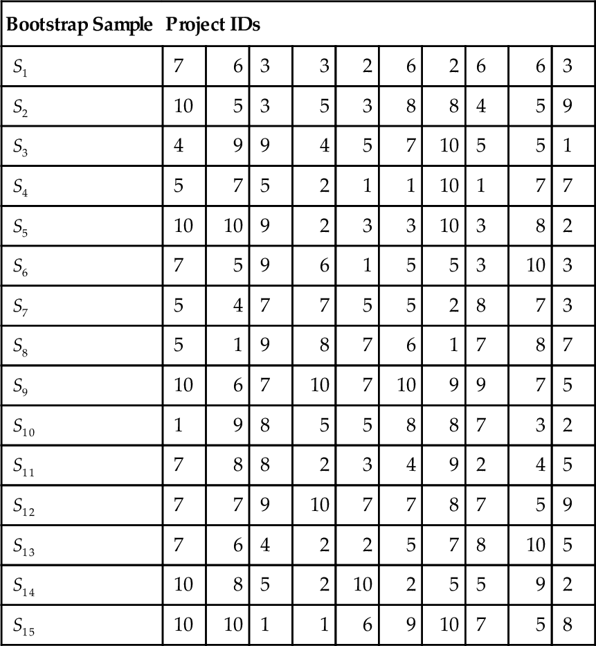
Only the project IDs are shown for simplicity.
After the ensemble is created, then it can start being used to make predictions for future instances based on their input features. In the case of SEE, future instances are new projects to which we do not know the true required effort and wish to estimate it. In the case of regression tasks, where the value to be estimated is numeric, the predictions given by the ensemble are the simple average of the predictions given by its base models. This would be the case for SEE. However, bagging can also be used for classification tasks, where the value to be predicted is a class. An example of classification task would be to predict whether a certain module of a software is faulty or nonfaulty. In the case of classification tasks, the prediction given by the ensemble is the majority vote, i.e., the class most often predicted by its base models.
20.2.2 When and why bagging works
The success of bagging depends on its base learning algorithm being unstable, where unstable means that a small change in the training sample can result in a large change in the predictions given by the resulting base model. It has been shown that bagging is able to improve the performance of good but unstable base learning algorithms. On the other hand, bagging could even slightly degrade the performance of stable base learning algorithms [46]. It has been pointed out that classification and RTs, neural networks, and subset selection in linear regression are typically unstable, whereas k-nearest neighbor is stable [46, 47].
The reason why bagging needs good but unstable base learning algorithms is related to accuracy and diversity (Section 20.1). If a stable base learning algorithm is used, then the predictions given by different base models created with different bootstrap samples of the training set will be very similar. A good but unstable base learning algorithm will create accurate but diverse base models, making bagging successful. In terms of the ambiguity decomposition explained in Section 20.1.2, good but unstable base learning algorithms would increase the ambiguity term, helping to reduce the error of the ensemble. Even if each of the base models is slightly less accurate than a single model trained on the whole training set, the reduction of the error caused by the ambiguity term would compensate for that. On the other hand, bagging using a stable base learning algorithm would not get its error reduced because the ambiguity term would be very small—in the extreme case, zero. At the same time, its base models may be slightly less accurate than single models trained on the whole data set would be. So, the error of the bagging ensemble could be slightly worse than single models trained on the whole training set if its base learners are stable.
20.2.3 Potential advantages of bagging for SEE
Bagging is a simple and well-known ensemble learning approach that has three main features that make it potentially beneficial for SEE: (1) several ready implementations of bagging can be easily found on the Web, (2) it does not require extensive human participation in the process of building ensembles, and (3) it has theoretically and empirically shown to improve performance in comparison to the base learning algorithm provided that its base learning algorithm is unstable enough [46].
20.3 Regression trees (RTs) for bagging
RTs were introduced earlier in this book (see Section 10.10). Such learners generate a tree of decisions whose leaves are a prediction for some numeric class (for example, see Figure 20.2).

In turns out that these kinds of tree learning are very useful for bagging. To see this, consider the following. As explained in Section 20.2, bagging uses a single type of base learning algorithm, which should allow for diversity to be produced, besides being accurate. Examples of learners that are typically unstable are RTs, neural networks, and subset selection in linear regression [46, 47]. In terms of accuracy, RTs have several potential advantages for SEE in comparison to other single learners, as explained in Section 10.10.5. Sections 20.5, 20.6 will confirm that RTs present relatively good performance and that their locality structure, which takes into account the difference in importance among input features, is key for their performance in SEE. The fact that RTs are typically unstable and accurate for SEE makes them good base learners for bagging in SEE. Our experimental study in Section 20.5 shows that bagging + RTs indeed present very competitive accuracy in SEE.
20.4 Evaluation framework
This chapter will present an experimental study with the aims of (1) evaluating bagging + RTs in comparison to several other fully automated ML approaches for SEE, and (2) providing further understanding on why bagging + RTs manage to obtain competitive performance in SEE. We refer to an approach as fully automated when, given the project data, it does not require human intervention and decision making in order to be used. This is an algorithmic feature that reduces the complexity and cost of using the SEE tool, as a person operating it would just need to provide the project data and push a button to obtain a SEE. It is worth noting that parameter choice can usually be automated as well. For instance, bagging + RT is an approach that can be fully automated.
Current work on frameworks for evaluation of SEE approaches considers issues such as explicit preprocessing [292], evaluation measures [133, 389], and the importance of the magnitude of the differences in performance [389]. There has also been work on statistical approaches for evaluating models across multiple data sets in the general ML literature [96]. In this section, we build upon existing work and present a framework that explicitly considers four important points: (1) choice of data sets and preprocessing techniques, (2) choice of learning machines, (3) choice of evaluation methods, and (4) choice of parameters. All these points should be considered carefully based on the aims of the experiments. The design chosen in this section concentrates mainly on the aim of evaluating (and choosing) ML models for SEE. Further design choices for providing additional understanding about why bagging + RTs obtain competitive performance are provided in Section 20.6.
20.4.1 Choice of data sets and preprocessing techniques
The first point in our framework is the choice of data sets and preprocessing techniques to be used in the study. Considering the aim of providing a general evaluation of a certain SEE approach in comparison to others, the data sets should cover a wide range of problem features, such as number of projects, types of features, countries, and companies. In this work, this is achieved by using five data sets from the PRedictOr Models In Software Engineering Software (PROMISE) Repository [300] and eight data sets based on the International Software Benchmarking Standards Group (ISBSG) Repository [271] Release 10. Sections 20.4.1.1, 20.4.1.2 provide their description and preprocessing.
20.4.1.1 PROMISE data
The PROMISE data sets used in this study are cocomo81, nasa93, nasa, sdr, and desharnais. Cocomo81 consists of the projects analyzed by Boehm to introduce COCOMO [34]. Nasa93 and nasa are two data sets containing Nasa projects from the 1970s to the 1980s and from the 1980s to the 1990s, respectively. Sdr contains projects implemented in the 2000s and was collected at Bogazici University Software Engineering Research Laboratory from software development organizations in Turkey. Desharnais' projects are dated from late 1980s. Table 20.4 provides additional details and the next paragraphs explain their features, missing values, and outliers.
Table 20.4
PROMISE Data Sets
| Data Set | # Projs | # Feats | Min Eff | Max Eff | Avg Eff | Std Dev Eff |
| Cocomo81 | 63 | 17 | 5.9 | 11,400 | 683.53 | 1821.51 |
| Nasa93 | 93 | 17 | 8.4 | 8211 | 624.41 | 1135.93 |
| Nasa | 60 | 16 | 8.4 | 3240 | 406.41 | 656.95 |
| Sdr | 12 | 23 | 1 | 22 | 5.73 | 6.84 |
| Desharnais | 81 | 9 | 546 | 23,940 | 5046.31 | 4418.77 |

Adapted from [326].
The effort is measured in person-months for all data sets but desharnais, where it is measured in person-hours. # Projs stands for number of projects, # Feats for number of features, and Eff for true required effort.
Features
Cocomo81, nasa93, and nasa are based on the COCOMO [34] format, containing as input features 15 cost, drivers, the number of lines of code (LOC) and the development type (except for nasa, which does not contain the latter feature). The actual effort in person-months is the dependent variable. Sdr is based on COCOMO II [37], containing as input features 22 cost drivers and the number of LOC. The actual effort in person-months is the dependent variable. The data sets were processed to use the COCOMO numeric values for the cost drivers. The development type was transformed into dummy variables.
Desharnais follows an independent format, containing as input features the team experience in years, the manager experience in years, the year the project ended, the number of basic logical transactions in function points, the number of entities in the system's data model in function points, the total number of nonadjusted function points, the number of adjusted function points, the adjustment factor, and the programming language. Actual effort in person-hours is the dependent variable.
Missing Values
The only data set with missing values is desharnais. In total, it contains only 4 in 81 projects with missing values. So, these projects were eliminated.
Outliers
The literature shows that SEE data sets frequently have a few outliers, which may hinder the SEEs for future projects [385]. In the current work, outliers were detected using k-means. This method was chosen because it has shown to improve performance in the SEE context [385]. K-means is used to divide the projects into clusters. The silhouette value for each project represents the similarity of the project to the other projects of its cluster in comparison to projects of the other clusters, ranging from −1 (more dissimilar) to 1 (more similar). So, the average silhouette value can be used to determine the number of clusters k. After applying k-means to the data, clusters with less than a certain number n of projects or projects with negative silhouette values are considered outliers.
We used n = 3, as in [385]'s work. The number of clusters k was chosen among k = {2, 3, 4, 5}, according to the average silhouette values. As shown in Table 20.5, the highest average silhouette values were always for k = 2 and were very high for all data sets (between 0.8367 and 0.9778), indicating that the clusters are generally homogeneous. The number of outliers was also small (from none to 3), representing less than 5% of the total number of projects, except for sdr. The projects considered as outliers were eliminated from the data sets, apart from the outlier identified for sdr. As this data set is very small (only 11 projects), there is not enough evidence to consider the identified project as an outlier.
Table 20.5
PROMISE Data Sets—Outliers Detection
| Data Set | K | Avg Silhouette | Outliers | # Outliers/# Projs |
| Cocomo81 | 2 | 0.9778 | None | 0.00% |
| Nasa93 | 2 | 0.9103 | 42, 46, 62 | 3.23% |
| Nasa | 2 | 0.9070 | 2, 3 | 3.33% |
| Sdr | 2 | 0.9585 | 9 | 8.33% |
| Desharnais | 2 | 0.8367 | 9, 39, 54 | 3.70% |

Adapted from [327].
The numbers identifying the outlier projects represent the order in which they appear in the original data set, starting from one. # Outliers stands for number of outliers and # Projs for the total number of projects in the data set.
20.4.1.2 ISBSG data
The ISBSG repository contains a large body of data about completed software projects. Release 10 contains 5052 projects, covering many different companies, several countries, organization types, application types, etc. The data can be used for several different purposes, such as evaluating the benefits of changing a software or hardware development environment; improving practices and performance; and estimation.
In order to produce reasonable SEE using ISBSG data, a set of relevant comparison projects needs to be selected. We preprocessed the data set to use projects that are compatible and do not present strong issues affecting their effort or sizes, as these are the most important variables for SEE. With that in mind, we maintained only projects with
• Data quality and function points quality A (assessed as being sound with nothing being identified that might affect their integrity) or B (appears sound but there are some factors that could affect their integrity; integrity cannot be assured).
• Recorded effort that considers only the development team.
• Normalized effort equal to total recorded effort, meaning that the reported effort is the actual effort across the whole life cycle.
• Functional sizing method IFPUG version 4+ or NESMA.
• No missing organization-type field. Projects with missing organization-type field were eliminated because we use this field to create different subsets, as explained in the next paragraph.
The preprocessing resulted in 621 projects.
After that, with the objective of creating different subsets, the projects were grouped according to organization type. Only the groups with at least 20 projects were maintained, following ISBSG's data set size guidelines. The resulting organization types are shown in Table 20.6. In addition, a data set containing the union of all the ISBSG subsets will also be used in our analysis, in order to create a data set likely to be more heterogeneous than the other ones.
Table 20.6
ISBSG Data—Organization Types Used in the Study
| Organization Type | ID | # Projs |
| Financial, Property, & Business Services | Org1 | 76 |
| Banking | Org2 | 32 |
| Communications | Org3 | 162 |
| Government | Org4 | 122 |
| Manufacturing, Transport, & Storage | Org5 | 21 |
| Ordering | Org6 | 22 |
| Billing | Org7 | 21 |
From [326].
# Projs stands for number of projects in the organization-type subset.
Table 20.7 contains additional information about the subsets. As we can see, the productivity rate of different companies varies. A 7-way 1-factor analysis of variance (ANOVA) [332] was used to determine whether the mean productivity rate for all different subsets are equal or not. The factor considered was organization type, with seven different levels representing each of the organization types, and each level containing its corresponding projects as the observations. ANOVA indicates that there is statistically significant difference at the 95% confidence interval (p-value < 2.2e–16).
Table 20.7
ISBSG Subsets
| ID | Min | Max | Avg | Std Dev |
| (a) Unadjusted function points | ||||
| Org1 | 43 | 2906 | 215.32 | 383.72 |
| Org2 | 53 | 499 | 225.44 | 135.12 |
| Org3 | 3 | 893 | 133.24 | 154.42 |
| Org4 | 32 | 3088 | 371.41 | 394.10 |
| Org5 | 17 | 13,580 | 1112.19 | 2994.62 |
| Org6 | 50 | 1278 | 163.41 | 255.07 |
| Org7 | 51 | 615 | 160.10 | 142.88 |
| (b) Effort | ||||
| Org1 | 91 | 134,211 | 4081.64 | 15, 951.03 |
| Org2 | 737 | 14,040 | 3218.50 | 3114.34 |
| Org3 | 4 | 20,164 | 2007.10 | 2665.93 |
| Org4 | 360 | 60,826 | 5970.32 | 8141.26 |
| Org5 | 762 | 54,620 | 8842.62 | 11, 715.39 |
| Org6 | 361 | 28,441 | 4855.41 | 6093.45 |
| Org7 | 867 | 19,888 | 6960.19 | 5932.72 |
| (c) Productivity | ||||
| Org1 | 1.2 | 75.2 | 12.71 | 12.58 |
| Org2 | 4.5 | 55.1 | 15.05 | 9.94 |
| Org3 | 0.3 | 43.5 | 17.37 | 9.98 |
| Org4 | 1.4 | 97.9 | 18.75 | 16.69 |
| Org5 | 2.2 | 52.5 | 23.38 | 14.17 |
| Org6 | 5.6 | 60.4 | 30.52 | 17.70 |
| Org7 | 14.4 | 203.8 | 58.10 | 61.63 |

Adapted from [326].
The next paragraphs explain how the features were selected and how to deal with the missing values and outliers.
Features
The ISBSG suggests that the most important criteria for estimation purposes are the functional size; the development type (new development, enhancement, or redevelopment); the primary programming language or the language type (e.g., 3GL, 4GL); and the development platform (mainframe, midrange, or PC). As the development platform has more than 40% missing feature values for two organization types, the following criteria were used as features:
• Development type.
• Language type.
The normalized work effort in hours is the dependent variable. Due to the preprocessing, this is the actual development effort across the whole life cycle.
Missing Values
The features “functional size” and “development type” have no missing values. The feature “language type” is missing in several subsets, even though it is never missing in more than 40% of the projects of any subset.
So, an imputation method based on k-nearest neighbors (k-NN) was used so that this feature can be kept without having to discard the projects in which it is missing. K-NN imputation has been shown to be able to improve SEEs [66]. It is particularly beneficial for this area because it is simple and does not require large data sets. Another method, based on the sample mean, also presents these features, but k-NN has been shown to outperform it in two SEE case studies [66].
According to [66], “k-NN works by finding the k most similar complete cases to the target case to be imputed where similarity is measured by Euclidean distance.” When k > 1, several different methods can be used to determine the value to be imputed; for example, simple average. For categorical values, vote counting is adopted. Typically, k = 1 or 2. As language type is a categorical feature, using k = 2 could cause draws. So, we chose k = 1. The Euclidean distance considered normalized data sets.
Outliers
Similarly to the PROMISE data sets (Section 20.4.1.1), outliers were detected through k-means [165] and eliminated. K was chosen among k = {2, 3, 4, 5} based on the average silhouette values. The best silhouette values, their corresponding ks, and the projects considered as outliers are shown in Table 20.8.
Table 20.8
ISBSG Subsets—Outliers Detection
| ID | K | Avg Silhouette | Outliers | # Outliers/# Projs |
| Org1 | 2 | 0.9961 | 38 | 1.32% |
| Org2 | 2 | 0.9074 | None | 0.00% |
| Org3 | 2 | 0.8911 | 80, 91, 103, 160 | 2.47% |
| Org4 | 2 | 0.8956 | 4, 10, 75, 89, 104 | 4.10% |
| Org5 | 2 | 0.9734 | 20 | 4.76% |
| Org6 | 3 | 0.8821 | 4 | 4.55% |
| Org7 | 3 | 0.8898 | None | 0.00% |

Adapted from [327].
The numbers identifying the outlier projects represent the order in which they appear in the original data set, starting from one. # Outliers stands for number of outliers and # Projs stands for number of projects in the organization type subset.
As with the PROMISE data sets, the silhouette values were high (between 0.8821 and 0.9961), showing that the clusters are homogeneous. The number of outliers varied from none to 5, representing always less than 5% of the total number of projects. None of the data sets were reduced to less than 20 projects after outliers elimination.
20.4.2 Choice of learning machines
The second point to be considered when designing a ML experiment is the approaches that will be included in the analysis. As explained in the beginning of Section 20.4, our design will concentrate on the aim of evaluating bagging + RTs against several other fully automated ML approaches. With that aim, three ensemble and three single fully automated learning machines were chosen to be used:
• Radial Basis Function (RBFs) networks [32]; and
• MultiLayer Perceptrons (MLPs) [32].
• Ensembles of learning machines:
• Bagging [46] with MLPs (bagging + MLPs), with RBFs (bagging + RBFs) and with RTs (bagging + RTs);
• Ensembles based on randomization [156, 444] of MLPs (randomizer + MLPs); and
• NCL [263, 264] with MLPs (NCL + MLPs).
RTs were chosen because they present several potential advantages for SEE, including their specific type of locality, as explained in Section 20.3. A study comparing different locality approaches, including the traditional SEE by analogy approach k-NN [390], and three clustering approaches, has shown that even though RTs obtained similar average ranking across data sets to the other locality approaches, when they were not the best, they rarely performed considerably worse than the best [326], being generally more adequate for SEE than the others.
RBFs were included because they are also learners based on locality, due to the RBFs (typically Gaussians) used in their hidden nodes. When the inputs are fed into the hidden layer, their distances (e.g., Euclidean distances) to the center of each neuron are calculated. After that, each node applies a RBF to the distance, which will produce lower/higher values for larger/shorter distances. Each hidden neuron i is connected to each output neuron j with weight wji, and output neurons usually compute a linear function of their inputs when working with regression problems. Due to the use of a RBF, changes in the weights connecting a given hidden neuron to the output neurons do not affect input values that are far from the center of this neuron.
Even though the choice of RTs and RBFs was based on their relation to locality, MLPs are not local learning machines and were included as an example of a nonlocal approach. They were chosen for being popular learning machines that can approximate any continuous function [32]. They have also been investigated in the SEE context [25, 45, 171, 242, 403, 422, 445]. For instance, Tronto et al. [422] showed that they can outperform linear regression because they are able to model observations that lie far from the best straight line. MLPs can be easily combined using several different ensemble approaches, such as bagging, random ensembles, and NCL. Other nonlocal approaches that are not restricted to certain function shapes were not chosen because they do not perform well for regression tasks (e.g., NaiveBayes [135]) or have not been so much used for SEE (e.g., support vector machines).
Bagging + RBFs and bagging + MLPs were also included to check whether other types of base learners could achieve similar performance to bagging + RTs.
Even though bagging is a well-known and accessible ensemble approach, each of its base learning machines is trained with only about 63.2% of the unique examples from the available original training set [26]. As the training data sets used for SEE are typically small, it is important to check whether using samples of the training set would not affect bagging badly in comparison to ensemble methods that train each of their base models with 100% of the training examples. So, our evaluation also included ensembles based on randomization of MLPs. They are based on the fact that different initial conditions may cause different neural networks to converge into different local minima of the cost function. They turn an apparent disadvantage, local minima in training neural networks, into something useful by averaging (in the case of regression) the predictions of base learning machines trained using different random seeds. Despite its simplicity, this procedure works surprisingly well in many, but not all, cases [92, 467, 468]. Their weakness is that a good level of diversity is not always achieved just by using different random seeds [264]. Note also that this approach can only be used with base learners that rely on random seeds, and are typically used with neural networks [421]. So, we used MLPs as their base learners in this study.
NCL [263, 264] is an ensemble approach that has strong theoretical foundations for regression problems, explicitly controlling diversity through the error function of the base learning machines [62]. So, it was also chosen to be included in the analysis. Its disadvantage is that its base models usually have to be very strong. Also, it can only be used with neural networks. Other learning machines such as RTs cannot be currently used. So, we used it with MLPs as the base learners in this study.
All the learning machines but NCL were based on the WEKA implementation [156, 444]. The RTs were based on the REPTree implementation available from Weka. We recommend the software WEKA [156, 444] should the reader wish to get more details about the implementation and parameters. The software used for NCL is available upon request.
20.4.3 Choice of evaluation methods
The third point in the experimental framework is the choice of evaluation methods. The evaluation was based on 30 runs for each data set. In each run, for each data set, 10 examples were randomly picked for testing and the remaining were used for the training of all the approaches being compared. Holdout of size 10 was suggested by Menzies et al. [292] and allows the largest possible number of projects to be used for training without hindering the testing. For sdr, half of the examples were used for testing and half for training, due to the small size of this data set.
The approaches are compared against each other based on their performance on the test set. Foss et al. [133] show that performance measures based on magnitude of the relative error (MRE) are potentially problematic due to their asymmetry, biasing toward prediction models that underestimate. That includes a performance measure very popular in the SEE literature: mean MRE (MMRE). Another measure, mean absolute error (MAE), does not present asymmetry problems and is not biased. However, it is difficult to interpret, as the residuals are not standardized. So, measures such as MMRE have continued to be widely used by most researchers in the area. However, Shepperd and Mc Donell [389] very recently proposed a new measure called standardized accuracy (SA), defined as follows:
where ![]() is the MAE of the prediction model Pi and
is the MAE of the prediction model Pi and ![]() is the mean value of a large number, typically 1000, runs of random guessing. This is defined as predicting
is the mean value of a large number, typically 1000, runs of random guessing. This is defined as predicting ![]() for the example t by randomly sampling over the remaining n − 1 examples and taking
for the example t by randomly sampling over the remaining n − 1 examples and taking ![]() , where r is drawn randomly with equal probability from 1 … n ^ r ≠ t. Even though this measure is a ratio, such as MMRE, this is not problematic because we are interested in a single direction—better than random [389]. SA can be interpreted as the ratio of how much better Pi is than random guessing, giving a very good idea of how well the approach does.
, where r is drawn randomly with equal probability from 1 … n ^ r ≠ t. Even though this measure is a ratio, such as MMRE, this is not problematic because we are interested in a single direction—better than random [389]. SA can be interpreted as the ratio of how much better Pi is than random guessing, giving a very good idea of how well the approach does.
The following measures of performance were used in this work [242, 292, 389]: MMRE, percentage of estimates within 25% of the actual values (PRED(25)), MAE, and SA. MMRE and PRED(25) were included for reference purposes, as they were reported in previous work evaluating ensembles [321]. In addition, verifying whether different results are achieved when using different performance measures can also provide interesting insights into the behavior of the approaches, as will be discussed in Section 20.5.4.
However, we will consider MAE and SA as more reliable performance measures. Unless stated otherwise, the analysis will always refer to the measures calculated on the test set.
As warned by Shepperd and Mc Donell [389], some papers in the SEE literature have been comparing approaches that do not perform better than random guess. To judge the effect size of the differences in performance against random guess, the following measure has been suggested:
where ![]() is the sample standard deviation of the random guessing strategy. The values of Δ can be interpreted in terms of the categories proposed by Cohen [80] of small (≈ 0.2), medium (≈ 0.5), and large (≈ 0.8). We use this measure to show how big the effect of the difference in MAE between each approach and random guess is likely to be in practice, validating our comparisons.
is the sample standard deviation of the random guessing strategy. The values of Δ can be interpreted in terms of the categories proposed by Cohen [80] of small (≈ 0.2), medium (≈ 0.5), and large (≈ 0.8). We use this measure to show how big the effect of the difference in MAE between each approach and random guess is likely to be in practice, validating our comparisons.
In order to determine whether the performance of the learning machines in terms of MAE is statistically significantly different from each other considering multiple data sets, we use the Friedman statistical test. Friedman was recommended by Demšar [96] as an adequate test for comparing multiple learning machines across multiple data sets. This statistical test also provides a ranking of algorithms as follows. Let rji be the rank of the jth of k algorithms on the ith of N data sets. The average rank of algorithm j is calculated as ![]() . The rounded average ranks can provide a fair comparison of the algorithms given rejection of the null hypothesis that all the approaches are equivalent. Nevertheless, Wilcoxon sign-rank tests [442] are typically used to compare a particular model to other models across multiple data sets after rejection of the Friedman null hypothesis, where necessary. Holm-Bonferroni corrections can be used to avoid high Type-I error due to the multiple tests performed.
. The rounded average ranks can provide a fair comparison of the algorithms given rejection of the null hypothesis that all the approaches are equivalent. Nevertheless, Wilcoxon sign-rank tests [442] are typically used to compare a particular model to other models across multiple data sets after rejection of the Friedman null hypothesis, where necessary. Holm-Bonferroni corrections can be used to avoid high Type-I error due to the multiple tests performed.
As data sets are very heterogeneous in SEE and the performance of the approaches may vary greatly depending on the data set, it is also important to check what approaches are usually among the best and, when they are among the worst, whether the magnitude of the performance is much worse than the best approach for that data set or not. This type of analysis also helps to identify for what type of data sets certain approaches behave better. It is worth noting that statistical tests such as Friedman and Wilcoxon are based on the relative ranking of approaches, thus not considering the real magnitude of the differences in performance when used for comparison across multiple data sets. So, even if a Friedman test accepts the null hypothesis that all approaches perform similarly across multiple data sets, it is still valid to check what approaches are most often among the best, on what type of data sets, and the magnitude of the differences in performance. In this work, we check the magnitude of the differences in performance between an approach and the best approach for a given data set by determining whether this approach has SA worse than the best in more than 0.1 units.
So, building upon previous work [96, 321, 389], an evaluation framework based on the following three steps is proposed by Minku and Yao (2012) [326]:
1. Friedman statistical test and ranking across multiple data sets to determine whether approaches behave statistically significantly differently considering several data sets.
2. Determine which approaches are usually among the first and second highest ranked approaches and, possibly, identify to which type of data sets approaches tend to perform better.
3. Check how much worse each approach is from the best approach for each data set.
A good approach would be highly ranked by Friedman and statistically significantly different from lower ranked approaches, would be more frequently among the best, and would not perform too bad in terms of SA when it is not among the best.
20.4.4 Choice of parameters
The fourth point considered in our framework is the choice of parameters for the approaches used in the experiments. The choice of parameters is a critical step in ML experiments, as results can vary greatly depending on it. For instance, a learning machine that would have better performance under certain choices could have worse performance under other choices. It is important that the method used for choosing the parameters is made clear in papers using ML, so that differences in the results obtained can be better understood.
In order to choose the parameters, we performed five preliminary runs using all combinations of the parameters shown in Table 20.9 for each data set and learning approach. The parameters providing the lowest MMRE for each data set were chosen to perform the thirty runs used in the comparison analysis. In this way, each approach enters the comparison using the parameters that are most likely to provide the best results for each particular data set. These parameters were omitted due to the large number of combinations of approaches and data sets used. The performance measure MMRE was chosen for being used in all previous work evaluating existing automated ensembles.
Table 20.9
Parameter Values for Preliminary Executions

From [326].
20.5 Evaluation of bagging + RTs in SEE
This section mainly aims at evaluating bagging + RTs in comparison to other automated ML approaches in SEE. As a preanalysis, we can observe that very different performances were obtained by the approaches for different data sets as follows. The MMRE obtained by the best performing approach for each particular data set varied from 0.37 to 2.00. The PRED(25) varied from 0.17 to 0.55. The correlation between estimated and real effort varied from 0.05 to 0.91. The SA varied from 0.26 to 0.64. Table 20.10 shows the SA and effect size Δ in comparison to random guess obtained by the approach with the highest, second highest, and lowest SA for each data set.
Table 20.10
SA and Effect Size Δ for Approaches Ranked as First, Second, and Last in Terms of SA for Each Data Set
| Approach | SA | Δ | |
| Cocomo81 | Bagging + MLP | 0.5968 | 0.9679 |
| RT | 0.5902 | 0.9572 | |
| RBF | 0.3024 | 0.4904 | |
| Nasa93 | RT | 0.6205 | 1.2647 |
| Bagging + RT | 0.6167 | 1.2569 | |
| NCL | 0.1207 | 0.2460 | |
| Nasa | Bagging + RT | 0.6423 | 1.5401 |
| RT | 0.6409 | 1.5367 | |
| RBF | 0.2618 | 0.6277 | |
| Sdr | RT | 0.2626 | 0.7508 |
| Bagging + RT | 0.2066 | 0.5907 | |
| Randomizer + MLP | −2.9981 · 108 | −1.3140 · 108 | |
| Desharnais | Bagging + MLP | 0.5248 | 1.7132 |
| Bagging + RT | 0.5049 | 1.6484 | |
| RBF | 0.3724 | 1.2157 | |
| Org1 | MLP | 0.4573 | 0.6670 |
| Bagging + MLP | 0.4441 | 0.6478 | |
| RT | 0.2245 | 0.3275 | |
| Org2 | Bagging + RBF | 0.2719 | 0.9941 |
| Bagging + MLP | 0.2716 | 0.9930 | |
| NCL | 0.0280 | 0.1025 | |
| Org3 | Bagging + RT | 0.5511 | 1.3237 |
| RT | 0.5347 | 1.2843 | |
| NCL | 0.4331 | 1.0402 | |
| Org4 | MLP | 0.3276 | 0.6995 |
| RBF | 0.3175 | 0.6779 | |
| NCL | 0.0248 | 0.0530 | |
| Org5 | Bagging + RT | 0.4259 | 1.9993 |
| Bagging + MLP | 0.4038 | 1.8957 | |
| NCL | 0.2117 | 0.9939 | |
| Org6 | Bagging + RBF | 0.4930 | 2.2358 |
| MLP | 0.4680 | 2.1224 | |
| NCL | 0.3617 | 1.6405 | |
| Org7 | Bagging + RBF | 0.3017 | 1.3739 |
| Bagging + MLP | 0.2948 | 1.3425 | |
| RBF | 0.0285 | 0.1300 | |
| OrgAll | Bagging + RT | 0.4416 | 1.0523 |
| RT | 0.4318 | 1.0288 | |
| Bagging + MLP | 0.3319 | 0.7907 |

Adapted from [326].
20.5.1 Friedman ranking
As a first step of the evaluation, the Friedman ranking of the ensembles, single learning machines, and random guess in terms of MAE was determined and the Friedman statistical test was used to check whether these approaches have statistically significantly different MAE. The ranking generated by the test is shown in Table 20.11. The Friedman test rejects the null hypothesis that all approaches perform similarly (statistic Ff = 12.124 > F(8, 96) = 2.036). As we can see from the table, random guess was always ranked last. An additional test was performed without including random guess and the null hypothesis was also rejected (statistic Ff = 4.887 > F(7, 84) = 2.121).
Table 20.11
Friedman Ranking of Approaches in Terms of MAE
| Rounded Avg. Rank | Avg. Rank | Std. Dev. Rank | Approach |
| 3 | 2.77 | 1.69 | Bagging + RT |
| 3.38 | 2.18 | Bagging + MLP | |
| 3.46 | 1.98 | Bagging + RBF | |
| 4 | 4.15 | 2.58 | RT |
| 5 | 4.54 | 2.22 | MLP |
| 5.23 | 1.54 | Randomizer + MLP | |
| 6 | 5.92 | 2.02 | RBF |
| 7 | 6.54 | 1.66 | NCL + MLP |
| 9 | 9.00 | 0.00 | Random Guess |

Adapted from [326].
All bagging approaches performed comparatively well, being on average ranked third. RTs were ranked on average just below, as fourth. As the null hypothesis that all approaches perform similarly was rejected, Wilcoxon sign-rank tests with Holm-Bonferroni corrections were performed to determine whether the RT's MAE is similar or different from bagging + RT's, bagging + MLP's, and bagging + RBF's across multiple data sets. Table 20.12 shows the p-values. The tests reveal that ensembles in general do not necessarily perform better than an adequate locality approach such as RTs. Bagging + MLP and bagging + RBF obtained statistically similar performance to RTs. However, bagging + RT, which is an ensemble of locality learning machines, obtained higher and statistically significantly different Friedman ranking in terms of MAE from single RTs. The number of win/tie/loss of bagging + RT versus RT is 10/1/2, further confirming the good performance of bagging + RTs, and demonstrating that RTs do not provide enough instability to allow bagging to improve upon its base learning algorithm only very rarely.
Table 20.12
Wilcoxon Sign-Rank Tests for Comparison of RT's MAE to Bagging + RT's, Bagging + MLP's, and Bagging + RBF's Across Multiple Data Sets
 |

Adapted from [326].
The p-value in light grey background represents statistically significant difference with Holm-Bonferroni corrections at the overall level of significance of 0.05.
Even though single RBFs use locality, they did not perform so well. A possible reason for that is that, even though locality is used in the hidden nodes, the output nodes are based on linear functions.
20.5.2 Approaches most often ranked first or second in terms of MAE, MMRE and PRED(25)
As a second step of the evaluation, the learning machines most often ranked as first or second in terms of MAE, MMRE, and PRED(25) were determined. Some results in terms of SA are also presented in order to provide more easily interpretable results.
In order to check how valid this analysis is, we first compare the SA and effect size Δ of the approach ranked as first, second, and last in terms of MAE for each data set. Table 20.10 shows these values. As we can see, the approaches ranked first or second frequently achieved SA at least 0.20 higher (better) than the worst approaches. That is reflected in the overall average SA considering all data sets, which improves from 0.2251 (approaches ranked last) to 0.4599 and 0.4712 (approaches ranked first and second). The effect size Δ in relation to random guess was frequently changed from small/medium to large, emphasizing the importance of using higher ranked approaches. Wilcoxon rank-sum statistical tests using Holm-Bonferroni corrections at the overall level of significance of 0.05 for comparing the approaches ranked first and second against random guess detected statistically significant difference for all cases. The p-values were very low, ranging from 1.6492 · 10−4 to 5.6823 · 10−19, confirming that the performance of these approaches is indeed better than random guessing.
Table 20.13a shows the learning machines ranked most often as first or second in terms of MAE. The results show that bagging + RTs, bagging + MLPs, and RTs are singled out, appearing among the first two ranked approaches in 27%, 23%, and 23% of the cases, whereas all other approaches together sum up to 27% of the cases. It is worth noting that bagging + RBF, which achieved high Friedman rank, does not appear so often among the best two approaches. One might think that bagging + RBFs rank for each data set could be more median, but more stable. However, the standard deviation of the ranks (Table 20.11) is similar to bagging + RTs and bagging + MLPs. So, the latter approaches are preferable over bagging + RBFs.
Table 20.13
Number of Data Sets in Which Each Learning Machine was Ranked First or Second According to MAE, MMRE, and PRED(25)
| PROMISE Data | ISBSG Data | All Data |
| (a) According to MAE | ||
| RT: 4 | Bagging + MLP: 4 | Bagging + RT: 7 |
| Bagging +RT: 4 | Bagging + RT: 3 | RT: 6 |
| Bagging + MLP: 2 | Bagging + RBF: 3 | Bagging + MLP: 6 |
| MLP: 3 | MLP: 3 | |
| RT: 2 | Bagging + RBF: 3 | |
| RBF: 1 | RBF: 1 | |
| (b) According to MMRE | ||
| RT: 4 | RT: 5 | RT: 9 |
| Bagging + MLP: 3 | Bagging + MLP 5 | Bagging + MLP: 8 |
| Bagging + RT: 2 | Bagging + RBF: 3 | Bagging + RBF: 3 |
| MLP: 1 | MLP: 1 | MLP: 2 |
| Rand + MLP: 1 | Bagging + RT: 2 | |
| NCL + MLP: 1 | Rand + MLP: 1 | |
| NCL + MLP: 1 | ||
| (c) According to PRED(25) | ||
| Bagging + MLP: 3 | RT: 5 | RT: 6 |
| Rand + MLP: 3 | Rand + MLP: 3 | Rand + MLP: 6 |
| Bagging + RT: 2 | Bagging + MLP: 2 | Bagging + MLP: 5 |
| RT: 1 | MLP: 2 | Bagging + RT: 3 |
| MLP: 1 | RBF: 2 | MLP: 3 |
| Bagging + RBF: 1 | RBF: 2 | |
| Bagging + RT: 1 | Bagging + RBF: 1 | |

Adapted from [326].
Learning machines never among the first or second are omitted.
The table also shows that RTs are comparatively higher ranked for PROMISE than for ISBSG, achieving similar ranking to bagging approaches for PROMISE, but lower ranking for ISBSG. Even though RTs perform statistically similarly to bagging + MLPs and bagging + RBFs (Section 20.5.1), the difference in performance is statistically significant in comparison to bagging + RTs. Further, Wilcoxon sign-rank tests to compare RTs and bagging + RTs considering separately PROMISE and ISBSG data show that there is no statistically significant difference considering PROMISE on its own (p-value 1), but there is considering ISBSG (p-value 0.0078). So, approaches joining the power of bagging ensembles to the locality of RTs may be particularly helpful for more heterogeneous data.
Table 20.13b shows the two learning machines most often ranked as first and second in terms of MMRE. Both RTs and bagging + MLPs are very often among the first two ranked learning machines according to MMRE. The trend can be observed both in the PROMISE and ISBSG data sets. For PROMISE, RTs, or bagging + MLPs appear among the first two ranked approaches in 70% of the cases, whereas all other learning machines together sum up to 30%. For ISBSG, RTs, or bagging + MLPs appear among the first two ranked in 62.5% of the cases, whereas all other learning machines together sum up to 37.5%. Wilcoxon sign-rank tests show that these two approaches perform similarly in terms of MMRE (p-value of 0.2439).
The analysis considering PRED(25) shows that both RTs and bagging + MLPs are again frequently among the first two ranked (Table 20.13c), but randomizer + MLP becomes more competitive. If we consider PROMISE data by itself, ensembles such as bagging + MLPs are more frequently ranked higher than single learning machines, even though that is not the case for ISBSG. However, a Wilcoxon sign-rank test across multiple data sets shows that bagging + MLPs and RTs are statistically similar in terms of PRED(25) (p-value of 0.7483). Tests considering PROMISE and ISBSG data separately do not find statistically significant difference either (p-value of 0.8125 and 0.3828, respectively).
As we can see, RTs and bagging + MLPs are singled out as more frequently among the best both in terms of MMRE, PRED(25) and MAE and they perform statistically similarly independent of the performance measure. Other approaches such as randomizer + MLP and bagging + RTs become more or less competitive depending on the performance measure considered. Bagging + RBFs, differently from the Friedman ranking, is not singled out, i.e., it is not frequently among the best. Our study also shows that bagging + RTs outperform RTs in terms of MAE mainly for ISBSG data sets, which are likely to be more heterogeneous.
20.5.3 Magnitude of performance against the best
In this section, we analyze how frequently an approach is worse than the best MAE approach in more than 0.1 units of SA. There are 34 cases in which approaches are worse than the best MAE approach of the data set in more than 0.1 units of SA. p-values of Wilcoxon tests to compare these approaches to the best MAE are below 0.05 in 28 cases. If we apply Holm-Bonferroni corrections considering all the 34 comparisons, the difference is statistically significant in 20 out of 34 cases (59%). So, it is reasonable to consider the number of times that each approach is worse than the best in order to evaluate its performance.
Table 20.14 shows how many times each approach is worse than the best MAE approach in more than 0.1 units of SA. As we can see, RTs and bagging + RTs are rarely worse than the best MAE approach in more than 0.1 SA. They are worse in only 1 in 13 data sets. Bagging + MLPs, bagging + RBFs, and MLPs behave slightly worse, with the difference in SA higher than 0.1 SA in 3 data sets.
Table 20.14
Number of Times That an Approach is Worse than the Best MAE Approach of the Data Set in More than 0.1 Units of SA
| Approaches | Number of Times |
| RT, Bagging + RT | 1 |
| Bagging + MLP, Bagging + RBF, MLP | 3 |
| Randomizer + MLP | 5 |
| RBF | 8 |
| NCL + MLP | 10 |
Adapted from [326].
20.5.4 Discussion
The analyzes presented in Sections 20.5.1, 20.5.2, and 20.5.3 show that bagging + RTs present a very good behavior for SEE. They have higher average (Friedman) rank, are more frequently among the best in terms of MAE, and are rarely worse than the best MAE approach for each data set in more than 0.1 units of SA. This is an example of how joining the power of bagging ensembles to a good locality approach can help improving SEE. Bagging + RTs were particularly helpful to improve performance in terms of MAE for ISBSG data sets, which are likely to be more heterogeneous. Future research on improving SEE using automated learning machines may benefit from further exploiting the advantages of ensembles and locality together.
As no approach is always the best independent of the data set, ideally, an organization should perform experiments following a principled framework in order to choose a model for their particular data set. Nevertheless, if an organization has no resources to perform such experiments, bagging + RTs are more likely to perform comparatively well across different data sets and are rarely worse than the best approach for a particular data set in more than 0.1 SA. Even though single RTs may perform slightly worse than bagging + RTs, they perform comparatively well in comparison to other approaches and may be used if the practitioners would like to understand the rules used by the learning machine to perform estimations.
The conclusions above are mainly drawn based on MAE and SA, which are considered to be more adequate and reliable performance measures than MMRE and PRED(N). In terms of behavior independent of the performance measure used, RTs and bagging + MLPs are always singled out as being frequently first or second ranked, whereas bagging + RT is less frequently among the best in terms of MMRE and PRED(25). Such a difference in the evaluation based on MAE and MRE-based measures gives us an interesting insight. It suggests that the slightly worse performance of RTs and bagging + MLPs in comparison to bagging + RTs in terms of MAE may be related to the fact that RTs and bagging + MLPs suffer more from underestimations. This issue should be further analyzed as future work and could be helpful for improving the performance of these approaches for SEE.
It is also worth making a note on the preprocessing of the data sets. As explained in Section 20.4.1, data sets were preprocessed using k-means for outliers removal. Outliers are examples different from usual and that cannot be well estimated by the models generated. Experiments done using RTs and bagging + MLPs reveal that the error obtained when attempting to use the models to estimate solely outlier projects is worse than the average obtained using nonoutlier examples, both in terms of MAE and PRED(25). Interestingly, the error in terms of MMRE is not much affected. As MMRE tends to bias models toward underestimations [389], these outliers are likely to be projects underestimated by the models.
We have also repeated the experiments using bagging + RTs, bagging + MLPs, and RTs, but without performing this part of the preprocessing, i.e., allowing the train/test sets to contain outliers. The experiments reveal that the SAs obtained are considerably reduced. So, in practice, the use of a clustering approach such as k-means is recommendable to remove outliers from the training sets and to identify whether a test example is an outlier.
20.6 Further understanding of bagging + RTs in SEE
Section 20.2 provides a clear explanation on why ensembles such as bagging using unstable base learners can perform well. Section 20.5 then shows that bagging + RTs only very rarely do not manage to outperform RTs. So, the amount of instability provided by RTs is enough for most SEE data sets investigated in this study. This explains part of the reason why bagging + RTs were successful. The other feature that makes an ensemble such as bagging successful is the accuracy of its base models. We will consider here MAE as the most appropriate measure for the analysis. As shown in Section 20.5, even though RTs did not perform as well as bagging + RTs, they obtained comparatively good performance in comparison to several other approaches and rarely performed worse than the best approach for a given data set in more than 0.1 units of SA. They have also allowed bagging + RTs to obtain in general better results in terms of MAE than bagging + MLPs and bagging + RBFs. So, we can consider RTs as accurate base learners for SEE. In order to provide a further understanding on why bagging + RTs performed well, we thus need to provide a further understanding on why RTs performed well.
As explained in Section 20.3, one of the key potential advantages of RTs over other approaches is that they perform not only feature selection, but also naturally consider and use the relative importance of input features. In order to confirm that the relative importance is one of the keys to RT's performance, we analyze in this section whether the separation of features provided by RTs provides better performance than using solely feature selection.
A correlation-based feature selection (CFS) method [154] with greedy stepwise search [156] was used in the analysis. This method was chosen because it uses a similar idea to RTs to check what features are more significant. It additionally checks the correlation among features themselves. Greedy stepwise search was used because it allows ranking features. The main reason for using this CFS is its similarity to the working of RTs, with the key difference that simply using its selected features as inputs for a learning machine does not provide it with a hierarchy of relative importance of the features. So, CFS is particularly helpful for understanding the behavior of RTs and how beneficial its use of the relative importance of features is to SEE. This filter method was also used instead of a wrapper method so that the same set of features can be used for different models, as explained below.
As a first step, we ran all the experiments using the design presented in Section 20.4, but after performing feature selection. This study showed that feature selection by itself did not change the fact that RTs and bagging + MLPs were usually among the best in terms of MMRE, PRED(25), and MAE. The approaches that obtained most improvements in performance were bagging + RBF, RBF, and NCL. However, the improvements were not large even for these approaches. Bagging + RBF's SA average considering all data sets was 0.0522 higher, RBF's was 0.0533, and NCL's was 0.0484 higher than when not using features selection.
As a second step for this analysis, we compared the ranking of features given by feature selection against the features appearing in more than 50% of the RTs until their third level, for each data set. An example is shown in Table 20.15. The results show that (1) the RTs do not use all the features selected by CFS, even though they usually use at least one of these; (2) the RTs use some features not selected by CFS; and (3) the RTs put higher ranked features according to CFS in higher levels of the tree, confirming the use of the relative importance of features.
Table 20.15
CFS Ranking and RT Features Relative Importance for cocomo81: Features Ranking, First Tree Level in Which the Feature Appeared in More than 50% of the Trees, and Percentage of the Trees in Which it Appears in That Level
| Features Ranking | Tree Level | % of Trees |
| LOC | Level 0 | 100.00% |
| Development mode | ||
| Required software reliability | Level 1 | 90.00% |
| Modern programming practices | ||
| Time constraint for cpu | Level 2 | 73.33% |
| Database size | Level 2 | 83.34% |
| Main memory constraint | ||
| Turnaround time | ||
| Programmers' capability | ||
| Analysts' capability | ||
| Language experience | ||
| Virtual machine experience | ||
| Schedule constraint | ||
| Application experience | Level 2 | 66.67% |
| Use of software tools | ||
| Machine volatility | ||
| Process complexity |
From [326].
Features below the horizontal line are not selected by CFS.
So, feature selection by itself was not able to change the relative performance of different learning approaches. However, instead of simply using a subset with the most important features, RTs gave more importance to more important features as shown by the feature ranking, being able to achieve comparatively good performance and showing that hierarchy of features is important when working with ML for SEE. Future approaches tailored to SEE may be able to improve performance further by combining the power of ensembles to good locality features such as the hierarchy of features used by RTs.
It is also interesting to verify which features are usually at the top level of the hierarchy produced by the RTs, as these are considered to be the most influential features for the SEE. The number of LOC and the functional size are the features that most frequently appear at the top level. Table 20.15 shows an example for cocomo81, for which 100% of the RTs used LOC at the top level (level 0). It is reasonable that this feature appears at the top of the hierarchy, as larger programs require involvement of many programmers, increasing the communication complexity and effort.
Nasa93 was the only data set where a feature other than LOC or functional size appeared at the top level in more than 50% of the RTs. For this data set, 100% of the RTs used the feature CPU time constraint at the top level. Interestingly, even though nasa and nasa93 are two data sets from the same organization, the RTs did not use the same feature at the top level for these two data sets. For nasa, 96.67% of the RTs used LOC at the top level. In order to better understand why this happened, we analyzed the values of the feature CPU time constraint for these two data sets. As shown in Table 20.16, the standard deviation of this feature for nasa93 is much higher than that for nasa. A Levene test [250] shows that the difference in variance is statistically significant (p-value of 0.0036). This indicates that CPU time constraint varies more for nasa93 than for nasa. Very different CPU time constraints are likely to directly affect the difficulty of the software development, thus considerably influencing its required effort. For example, extra high CPU time constraint should require much more effort than low CPU time constraint. So, it is reasonable that this is considered as an important feature for nasa93.
Table 20.16
CPU Time Constraint Information
| Data Set | Minimum | Maximum | Avg | Std. Dev |
| Nasa93 | 1.00 | 1.66 | 1.133 | 0.203 |
| Nasa | 1.00 | 1.66 | 1.076 | 0.138 |

From [326].
It is also worth noting that the nonfunctional system features that are becoming more important in the modern systems could also affect the hierarchy provided by the RTs. For example, as writing secure code becomes more important for some companies, security-related features may raise in the hierarchy.
20.7 Summary
This chapter presents a didactic explanation of ensembles, in particular bagging; a principled and comprehensive evaluation of bagging + RTs for SEE; and an explanation of why bagging + RTs perform well in SEE. An additional contribution of this chapter is a principled framework for evaluating SEE approaches, which considers explicitly the choice of data sets and preprocessing techniques, learning approaches, evaluation methods, and parameters.
Bagging + RTs are shown to perform well in terms of MAE (and SA): they were highly ranked in terms of performance across multiple data sets, they were frequently among the best approaches for each data set, and rarely performed considerably worse than the best approach for any data set. Overall, they performed better than several other approaches. This is an encouraging result, specially considering that bagging + RTs are accessible and fully automated approaches. If an organization has no resources to perform experiments to choose the SEE approach that is most suitable to their own data, bagging + RTs are recommended for the reasons above. Even though RTs performed slightly worse than bagging + RTs, they could still be used should the software manager wish to easily understand the rules underlying the model's behavior.
The good results provided by bagging + RTs are obtained thanks to the successful combination of bagging, which can improve performance of diverse and accurate base models, to the success of RTs in SEE, which can create accurate base models through its locality based on hierarchy of features. Other approaches further exploiting ensembles and locality, in particular the use of a hierarchy of input features, may be able to improve SEE further.