
How To Keep Your Data Private
Abstract
In this part of the book Data Science for Software Engineering: Sharing Data and Models, we show that sharing all data is less useful that sharing just the relevant data. There are several useful methods for finding those relevant data regions including simple nearest neighbor, or kNN, algorithms; clustering (to optimize subsequent kNN); and pruning away “bad” regions. Also, we show that with clustering, it is possible to repair missing data in project records.
| Name: | CLIFF&MORPH |
| Also known as: | CLIFF is an instance selector that can be used as an instance-based selector (or case-based) reasoner. MORPH is an instance mutator and can also be categorized as a noise injector. |
| Intent: | The combination of CLIFF&MORPH is used as a privacy algorithm for software defect prediction when there is insufficient local data to build a defect predictor. |
| Motivation: | There are promising results with cross-company defect prediction (CCDP), however CCDP requires data sharing, which raises privacy concerns. Can minimizing the data with CLIFF and privatizing the remaining data with MORPH maintain the promising results while providing adequate privacy? |
| Solution: | For defect data, CLIFF seeks those instances that best predict for the target class. For each class value (“defective” and “nondefective”) we measure the frequency of an attribute value for one class value versus the other class value(s). We call these measures ranks and calculate them for each attribute value. We then find the products of these ranks for each instance, and those instances with the lowest ranks are discarded. MORPH's goal is to minutely change the values of data to protect it while keeping it useful for defect prediction. |
| Applicability: | CLIFF&MORPH was successful for CCDP: that is, with these tools, we can privatize data while keeping it useful. |
| Related to: | The research described in this chapter is the first known for privacy in CCDP. It shows that data can be made private and remain useful. This is especially important in a field of study such as CCDP, where data sharing is a requirement. |
This chapter is an update to “Balancing Privacy and Utility in Cross-Company Defect Prediction” by F. Peters, T. Menzies, L. Gong, and H. Zhang, which was published in the IEEE Transactions on Software Engineering, August 2013. This chapter extends that work with a practitioner focus. Sections 16.2–16.5 expand on topics such as “what is privacy-preserving data publishing?” and a review of how and why the background knowledge of an attacker can be integrated as a part of privacy measures.
16.1 Motivation
Data sharing is the enemy of privacy preservation. In the wrong hands shared data can lead to an individual's identity being stolen, loans and health insurance coverage can be denied, and an individual can become a victim of financial fraud. However, in the right hands, terrorists can be identified, scientists find treatments that work better than others, and doctors are aided in treatment and diagnostic decisions. So, to minimize the problems that can be caused by attackers (those seeking to gain confidential knowledge about individuals), the new and active fields of privacy preserving data publishing (PPDP) and privacy preserving data mining (PPDM) have been developed.
Researchers in PPDP and PPDM have disclosed their concerns of an attackers' negative use of such a helpful tool. For instance, Wang et al. [436] wrote:
Recent development in privacy-preserving data mining has proposed many efficient and practical techniques for hiding sensitive patterns or information from been discovered by data mining algorithms.
Zhang and Zhao [456] also noted that although successful in many applications, data mining poses special concerns for private data. Other researchers [14, 161, 175, 258], have gone farther showing how easily an attacker could uncover an individual's private/confidential data using readily available data mining tools. So, in order to take advantage of the good that can result from data mining while protecting the privacy of individuals, researchers have come up with many privacy protection techniques in the areas of PPDP and PPDM.
PPDP covers methods and tools used to disguise raw data for publishing, while PPDM covers methods and tools used to limit the amount of extra information gained by an attacker after performing some data mining task on published data. In spite of their relatively short existence, there are a plethora of published privacy protecting techniques designed to address a number of different scenarios. Therefore, to narrow the scope of this chapter, we will focus on PPDP and the simple scenario of disguising one data set for publication.
In this chapter we answer the following questions:
• What is PPDP and why is it important?
• What is considered a breach of privacy?
• How do you avoid privacy breaches?
• How are privacy preserving algorithms evaluated?
Finally, we conclude this chapter with a case study of privacy in cross-company defect prediction (CCDP) (Section 16.6).
16.2 What is PPDP and why is it important?
Similarly, researchers agree that PPDP involves the use of techniques to disguise the microdata records that contain information about specific individuals, while delivering a useful data set for analysis. This is indicated clearly by Fung et al. [138], who noted that PPDP is a collection of methods and tools for publishing data in a hostile environment so that the published data remains practically useful while individual privacy is preserved. Along the same lines, Domingo-Ferrer and Gonzalez-Nicolas [104] states:
Statistical disclosure control (also known as privacy-preserving data mining) of micro-data is about releasing data-sets containing the answers of individual respondents protected in such a way that: (i) the respondents corresponding to the released records cannot be re-identified; (ii) the released data stay analytically useful.
Also, according to LeFevre et al. [247], protecting individual privacy is an important problem in microdata distribution and publishing. Anonymization (privacy) algorithms typically aim to satisfy certain privacy definitions with minimal impact on the quality of the resulting data.
The importance of PPDP can be answered with a question: What is data mining without data? However, privacy concerns can limit data sharing. For instance, when America on Line (AOL) released the query logs of its users for the purpose of research, Thelma Arnold was reidentified by the examination of query terms from the logs [22]. AOL removed the logs immediately.
Reidentification is sensitive attribute disclosure. This is where an individual in a data set can be associated with a sensitive attribute value. Consider the example in Figure 16.1. Here the shaded column represents the sensitive attribute values, while the other columns represent the quasi-identifiers (QIDs). QIDs are attributes that can potentially reidentify an individual record such as age, zip code, and birth date. (Please note that the names are only included for ease of explanation. Normally, these are removed before publication.)

So, let us consider Jenny. In order for an attacker (let's say Jenny's boss, Bill) to reidentify her in the data set, through casual investigation Bill can figure out that Jenny had a recent stay at the hospital. Furthermore, once he figures out Jenny's age, he will find Jenny's record with 100% certainty and realize that Jenny is HIV positive. Clearly, privacy breaches of this nature can lead, in Jenny's case, to being discriminated against. Other scenarios could involve identity theft, loans and health insurance coverage can be denied, and an individual can become a victim to financial fraud.
In this regard, the goal of privacy algorithms is to add uncertainty to the point where, if Bill only has access to the table in Figure 16.2, then he can only reidentify Jenny's record with 33% certainty; therefore, only know that there is a 33% chance that Jenny has HIV rather than being 100% sure (Figure 16.1).

Ever-increasing data collection has led to privacy concerns [429]. The examples above show justification for such concerns. In the remainder of this chapter we aim to show that given some trade-off between privacy and utility or the usefulness of data, we can limit the occurrences of the examples above.
16.3 What is considered a breach of privacy?
In order to discover privacy breaches, one needs to define what constitutes a privacy breach for a particular data set. There are different levels of privacy. Some levels are determined by individuals in the data set or by the creators of a privacy policy or laws. An optimal result of a privacy model is defined by Dalenius [89] where he states that access to published data should not enable the attacker to learn anything extra about any target victim, compared to no access to the database, even with the presence of any attacker's background knowledge obtained from other sources [138].
Fung et al. [138], considers two categories of privacy models:
1. A privacy threat occurs when an attacker is able to link a record owner to a sensitive attribute in a published data table. These are specified as record linkage, attribute linkage, and table linkage, respectively.
2. The published data should provide the attacker with little additional information beyond his or her background knowledge.
Brickell and Shmatikov [57], defines a privacy model called sensitive attribute disclosure, which occurs when the attacker or adversary learns information about an individual's sensitive attributes. In other words, it captures the gain in the attacker's knowledge due to his/her observations of the disguised data set. Also, “Microdata privacy can be understood as prevention of membership disclosure,” where the attacker should not learn whether a particular individual is included in the database.
In 2007, Wang et al. [437] put forward other definitions of privacy. The article explains:
There have been two types of privacy concerning data mining. The first type of privacy, called output privacy, is that the data is minimally altered so that the mining result will not disclose certain privacy. The second type of privacy, called input privacy, is that the data is manipulated so that the mining result is not affected or minimally affected.
For the scenario used, we assume a privacy definition of high, where an attacker is unsuccessful at getting more information from the sanitized data set. The methods used to avoid privacy breaches are described in the following section.
16.4 How to avoid privacy breaches?
The idea of disguising a data set is known as anonymization. This is performed on the original data set to “satisfy a specified privacy requirement” [138] resulting in a modified data set being published. There are five general categories for anonymization: (1) generalization, (2) suppression, (3) anatomization, (4) permutation, and (5) perturbation. Most methods and tools created for preserving privacy fall into one or more of these categories and have some drawbacks.
Before we expand on the above categories, we repeat some definitions from Fung et al. [138]:
• The explicit identifier is a set of attributes, such as name and Social Security number, containing information that explicitly identifies record owners.
• The QID is a set of attributes that could potentially identify record owners.
• The sensitive attributes consists of sensitive person-specific information such as disease, salary, and disability status.
• The nonsensitive attributes contains all attributes that do not fall into the previous three categories.
16.4.1 Generalization and suppression
Many researchers comment on how privatization algorithms can distort data. For example, consider privatization via generalization and suppression. Generalization can be done by replacing exact numeric values with intervals that cover a subrange of values; e.g., 17 might become 15…20 or by replacing symbols with more general terms; e.g., “date of birth” becomes “month of birth.” Suppression can be done by replacing exact values with symbols such as a star or a phrase like “don't know” [433].
According to Fung et al. [138], generalization and suppression hide potentially important details in the QIDs that can confuse classification. Worse, these transforms may not guarantee privacy.
Widely used generalization and suppression approaches include k-anonymity, l-diversity, and t-closeness k-anonymity [412] makes each record in the table indistinguishable with k − 1 other records by suppression or generalization [353, 375, 412]. The limitations of k-anonymity, as listed by Brickell and Shmatikov [57], are many-fold. They state that k-anonymity does not hide whether a given individual is in the database. Also, in theory, k-anonymity hides uniqueness (and hence identity) in a data set, thus reducing the certainty that an attacker has uncovered sensitive information. However, in practice, k-anonymity does not ensure privacy if the attacker has background knowledge of the domain (see Figure 16.3). An example of k-anonymity in action and how background knowledge of an attacker can affect privacy is shown in Figure 16.3.

Machanavajjhala et al. [278] proposed l-diversity. The aim of l-diversity is to address the limitations of k-anonymity by requiring that for each QID group,1 there are at least l distinct values for each sensitive attribute value. In this way an attacker is less likely to “guess” the sensitive attribute value of any member of a QID group.
Work by Li and Li [255] later showed that l-diversity was vulnerable to skewness and similarity attacks, making it insufficient to prevent attribute disclosure. Hence, Li and Li proposed t-closeness to address this problem. t-Closeness focuses on keeping the distance between the distributions of a sensitive attribute in a QID group and that of the whole table no more than a threshold t apart. The intuition is that even if an attacker can locate the QID group of the target record, as long as the distribution of the sensitive attribute is similar to the distribution in the whole table, any knowledge gained by the attacker cannot be considered as a privacy breach because the information is already public. However, with t-closeness, information about the correlation between QIDs and sensitive attributes is limited [255] and so causes degradation of data utility.
16.4.2 Anatomization and permutation
Anatomization and permutation both accomplish a similar task; that is, the deassociation of the relationship between the QID and sensitive attributes. However, anatomization does it by releasing “the data on QID and the data on the sensitive attribute in two separate tables…” with “one common attribute, GroupID” [138]. On the other hand, permutation deassociates the relationship between a QID and a numerical sensitive attribute. This is done by partitioning a set of data records into groups and shuffling the sensitive values within each group [456].
16.4.3 Perturbation
A precise definition of perturbation is put forward by Fung et al. [138]:
The general idea is to replace the original data values with some synthetic data values, so that the statistical information computed from the perturbed data does not differ significantly from the statistical information computed from the original data.
It is important to note that the perturbed data records do not correspond to real-world record owners. Also, methods used for perturbation include additive noise, data swapping, and synthetic data generation. The drawback of these transforms is that they may not guarantee privacy. For example, suppose an attacker has access to multiple independent samples from the same distribution from which the original data was drawn. In that case, a principal component analysis could reconstruct the transform from the original to privatized data [142]. Here, the attacker's goal is to estimate the matrix (MT) used to transform the original data to its privatized version. MT is then used to undo the data perturbation applied to the original data. According to Giannella et al. [142], MT = WD0Z′, where W is the eigenvector matrix of the covariance matrix of the privatized data. Z′ is the transform of the eigenvector matrix of the covariance matrix of the independent samples. Finally, D0 is an identity matrix.
16.4.4 Output perturbation
Different than perturbation where the data is transformed to maintain its privacy, output perturbation maintains the original data in a database and instead adds noise to the output of a query [101]. Differential privacy falls into the category of output perturbation. Work by Dinur and Nissim [101] also falls into this category and forms the basis of Dwork's work on differential privacy [108, 109] (![]() -differential).
-differential).
According to Fung et al. [138], ![]() -differential privacy is based on the idea that the risk to the record owner's privacy should not substantially increase as a result of participating in a statistical database. So, instead of comparing the prior probability and the posterior probability before and after accessing the published data, Dwork [108, 109] proposed to compare the risk with and without the record owner's data in the published data.
-differential privacy is based on the idea that the risk to the record owner's privacy should not substantially increase as a result of participating in a statistical database. So, instead of comparing the prior probability and the posterior probability before and after accessing the published data, Dwork [108, 109] proposed to compare the risk with and without the record owner's data in the published data.
Dwork [108, 109] defines ![]() -differential privacy as follows:
-differential privacy as follows:
We say databases D1 and D2 differ in at most one element if one is a proper subset of the other and the larger database contains just one additional row.
Although ![]() -differential privacy assures record owners that they may submit their personal information to the database securely, it does not prevent membership disclosure and sensitive attribute disclosure studied in this work. This is shown in an example from Chin and Klinefelter [76] in a Facebook advertiser case study. Through reverse engineering, Chin and Klinefelter [76] inferred that Facebook uses differential privacy for its targeted advertising system. To illustrate the problem of membership and sensitive attribute disclosure, the authors described Jane's curiosity about her neighbor John's HIV status when she learned that he was on the finisher's list for the 2011 Asheville AIDS Walk and 5K Run. So, armed with John's age and zip code, she went to Facebook's targeted advertising area and found that there was exactly one male Facebook user age 36 from zip code 27514 who listed the “2011 Asheville AIDS Walk and 5K Run” as an interest. At this point, Jane placed a targeted advertisement offering free information to HIV-positive patients about a new antiretroviral treatment. If charged by Facebook for having her ad clicked, Jane can assume with some level of certainty that John is HIV positive.
-differential privacy assures record owners that they may submit their personal information to the database securely, it does not prevent membership disclosure and sensitive attribute disclosure studied in this work. This is shown in an example from Chin and Klinefelter [76] in a Facebook advertiser case study. Through reverse engineering, Chin and Klinefelter [76] inferred that Facebook uses differential privacy for its targeted advertising system. To illustrate the problem of membership and sensitive attribute disclosure, the authors described Jane's curiosity about her neighbor John's HIV status when she learned that he was on the finisher's list for the 2011 Asheville AIDS Walk and 5K Run. So, armed with John's age and zip code, she went to Facebook's targeted advertising area and found that there was exactly one male Facebook user age 36 from zip code 27514 who listed the “2011 Asheville AIDS Walk and 5K Run” as an interest. At this point, Jane placed a targeted advertisement offering free information to HIV-positive patients about a new antiretroviral treatment. If charged by Facebook for having her ad clicked, Jane can assume with some level of certainty that John is HIV positive.
16.5 How are privacy-preserving algorithms evaluated?
Three privacy evaluation methods are outlined in work by Torra et al. [418]. These measures are (1) information loss measures, (2) disclosure risk measures, and (3) scores. Information loss measures are designed to establish to which extent published data is still valid for carrying out the experiments planned on the original data. They take into account the similarity between the original data set and the protected one, as well as the differences between the results that would be obtained with the original data set and the results that would be obtained from the disguised data set. Torra et al. [418] further explain that disclosure risk measures are used to evaluate the extent in which the protected data ensures privacy and that scores is a summary of both information loss and disclosure risk; that is, when these two measures are commensurate, it is possible just to combine them using the average.
In the following sections we explain some of the privacy metrics used and how the attacker's background knowledge is used in these metrics.
16.5.1 Privacy metrics
Privacy metrics allows you to know how private the sanitized version of your data is. There are two categories of privacy metrics in the literature: syntactic and semantic [57]. The syntactic measures consider the distribution of attribute values in the privatized data set and are used by algorithms such as k-anonymity and l-diversity. In comparison, the semantic metrics measure what an attacker may learn or the incremental gain in knowledge caused by the privatized data set [57] and use distance measures such as the earth movers distance, KL divergence, and JS divergence to quantify this difference in the attackers knowledge. Other methods in the literature include increased privacy ratio (IPR) [355, 356], entropy [67, 79], and guessing anonymity [364, 413].
Previous privacy studies in software engineering (SE) [67, 79] have used entropy to measure privacy. Entropy (H) measures the level of uncertainty an attacker will have in trying to associate a target to a sensitive attribute. For example, if querying a data set produces two instances with the same sensitive attribute value then the attacker's uncertainty level or entropy is zero(0). However, if the sensitive attribute values are different, the attacker has a ![]() chance of associating the target with the correct sensitive attribute value. The entropy here is 1 bit, assuming that there are only two possible sensitive values. In general, the entropy of a data set is,
chance of associating the target with the correct sensitive attribute value. The entropy here is 1 bit, assuming that there are only two possible sensitive values. In general, the entropy of a data set is, ![]() bits, which corresponds to the number of bits needed to describe the outcome. Here, si is the probability that S = si.
bits, which corresponds to the number of bits needed to describe the outcome. Here, si is the probability that S = si.
Guessing anonymity was introduced by Rachlin et al. [364] and it is described as a privacy definition for noise perturbation methods. Guessing anonymity of a privatized record in a data set is the number of guesses that the optimal guessing strategy of the attacker requires to correctly guess the record used to generate the privatized record [364, 413].
We introduced IPR in previous work [355]. It is based on the adversarial accuracy gain, Aacc from the work of Brickell and Shamtikov [57]. According to the authors' definition of Aacc, it quantifies an attacker's ability to predict the sensitive attribute value of a target t. Aacc measures the increase in the attacker's accuracy after he observes a privatized data set and compares it to the baseline from a trivially privatized data set that offers perfect privacy by removing either all sensitive attribute values or all the other QIDs.
For IPR, we assume the role of an attacker armed with some background knowledge from the original data set and also supplied with the private data set. When the attacker predicts the sensitive attribute value of a target we use the original data to see if the prediction is correct. If it is we consider this as a privacy breach; otherwise, it is not. The IPR is the percentage of the total number of predictions that are incorrect. More specific details about IPR are in the Evaluating Privacy section of the case study later in this chapter (Section 16.6.8).
16.5.2 Modeling the background knowledge of an attacker
The attacker's background knowledge is an essential element of privacy metrics. Syntactic measures of privacy do not consider background knowledge; however, the semantic measures do. Incorporating the attacker's background knowledge is an active area of research [72, 106, 256, 257, 282]. These works measure the privacy risk when an attacker has a certain amount of knowledge. However, the major challenge facing you as the data owner, is that you're not a mind reader; you don't know the specific background knowledge of any attacker.
Martin et al. [282] provide one of the first methods for modeling an attacker's background knowledge. Their work does not assume that you know the attacker's background knowledge; instead, they assume bounds on the attacker's knowledge in terms of the number of basic units of knowledge of the attacker. In other words, the authors take the worst-case view where the attacker obtained the complete information about which individuals have records in the data set.
This work was then extended by Chen et al. [72]. They complained that the formal language developed by Martin et al. quantified background knowledge in a less than intuitive fashion. They also stated that because of this it would be difficult for you as the data owner to set an appropriate value for k which is the number of k, implications that an attacker may know. To improve on this, Chen et al. provide an intuitive, and therefore usable, quantification of an attacker's background knowledge. They consider three types of knowledge that arise naturally:
1. Knowledge about the target individual.
2. Knowledge about others.
3. Knowledge about same value families.
Li and Li [256] represented background knowledge as patterns or negative association rules that exist in the data. Unlike the work done by Martin et al. [282] and Chen et al. [72], this work lifts the burden from the user by not requiring the background knowledge as an input parameter. The authors believe that it should be possible to discover certain negative facts from the data such as, “male can never have ovarian cancer.” Further, such knowledge is helpful when privatizing data via grouping. An anonymization technique will avoid including ovarian cancer in any group including males.
Privacy-MaxEnt is a generic and systematic method to integrate background knowledge in privacy quantification. According to Du et al. [106], it can deal with many different types of background knowledge such as it is rare for males to have breast cancer, a probability or inequality, and that “Frank has pneumonia,” or “either Iris or Brian has lung cancer.” Du et al.'s work focuses mainly on distributional knowledge and states that most of this type of knowledge can be expressed using conditional probability. For example P(Breast Cancer|Male) = 0. So they formulate background knowledge as constraints and use maximal entropy modeling to derive the conditional probabilities between the QIDs and the sensitive attribute values [257].
In a later work by Li et al. [257], titled “Modeling and integrating background knowledge in data anonymization,” the authors presented a framework for modeling and computing background knowledge using kernel methods. The authors chose to use kernel regression method to approximate the probability distribution function; in other words, the attacker's prior knowledge or belief. Accordingly, this kernel estimation framework has three characteristics:
1. Focus on background knowledge that is consistent with the data.
2. Model background knowledge as probability distributions.
3. Use a kernel regression estimator to compute background knowledge.
All these studies about background knowledge have one thing in common: they acknowledge the difficulty in modeling an attacker's exact background knowledge. In addition, none can claim that they have addressed all types of background knowledge.
16.6 Case study: privacy and cross-company defect prediction
Software development produces many types of artifacts such as requirements, defect data, bug reports, and more. Privacy issues are dealt with differently for these different artifacts, and in this case study we focus on protecting the privacy of defect data used in CCDP.
Within-company defect prediction (WCDP) is the means by which organizations predict the number of defects in their software. CCDP looks at the feasibility of learning defect predictors using data from other companies. Recent studies show that defect and effort predictors built from cross-company data can be just as effective as predictors learned using within-company data [221, 427] (caveat: the cross-company data must be carefully filtered before being applied locally). This is potentially a very important result that implies the existence of general principles of SE (such generalities would lead us to general models of SE).
However, before we conduct widespread CCDP experiments, we must address the privacy concerns of data owners. Extracting data from organizations is often difficult due to the business sensitivity associated with the data. Because of this sensitivity, data owners who want to share limited amounts of useful data (say, to advance scientific research leading to improved software) need to do so without breaching any data privacy laws or company privacy policies.
For these reasons, many researchers doubt the practicality of data sharing for the purposes of research. In a personal communication, Barry Boehm reports he can release none of the data that his COCOMO team collected after 1981. Similarly, at a keynote address at ESEM'11, Elaine Weyuker doubted that she will ever be able to release the AT&T data she used to build defect predictors [440].
For companies with common concerns (e.g., subcontractors for a primary company), the benefits of sharing data can include improved software quality and reduced SE costs. Ideally, these organizations should be able to share data without revealing too much. Such organizations need to
1. Prevent the disclosure of specific sensitive metric values from their released data.
2. Ensure that the privatized data remain useful for research purposes, such as CCDP.
As shown below, standard methods such as k-anonymity do not protect against any background knowledge of an attacker (Table 16.1 defines this and other terms used in this study) and so may still reveal the sensitive attribute of a record. Moreover, two recent reports concluded that the more we privatize data, the less useful it becomes for certain utilities of certain tasks; for example, classification. Grechanik et al. [146] and Brickell and Shmatikov [57] reported that the application of standard privacy methods such as k-anonymity, l-diversity, and t-closeness damages inference power as privacy increases.
Table 16.1
Definitions of Terms Used in the Case Study (Section 16.6) of this Chapter
| Terms | Definitions |
| Classification |
• For a data set containing independent attributes and one dependent attribute (class) • We find a model for the dependent attribute as a function of the independent attributes • The goal is to assign the right class value to an unseen instance • Defect prediction is an example of a classification task |
| Class boundary | The border between neighboring regions of different classes |
| EFB | Equal frequency binning. EFB divides the range of possible values into n bins or subranges, each of which holds the same number of attribute values. If duplicate values are placed into different bins, boundaries of every pair of neighboring bins are adjusted so that duplicate values belong to one bin only [240] |
| CLIFF | An instance selection method |
| Power subrange | Power of each attribute subrange; i.e., how much more frequently that subrange appears in one class more than any other |
| MORPH | Data transformation via perturbation to create synthetic data |
| ti | A tuple of attribute values representing an individual record in a data set. Also referred to as a target in this work |
| T | Original data set containing targets |
| T′ | Privatized data set |
| T* | Represents either T or T′ |
| A | Set of attributes |
| ai | Attribute |
| t[ai] | The value of attribute ai for t |
| ID | Identifier—anything that specifically identifies an individual or thing such as a Social Security number |
| QIDs | Quasi-identifiers are attributes that can be used to reidentify an individual record in a data set. These attributes can also be sensitive |
| si | Sensitive attribute value |
| S | Set of possible sensitive attribute values that we do not want an attacker to associate with a target, t in a data set |
| qi | A query is made up of attribute value pair(s). Example q3 is “a1 = t[a1] and a2 = t[a2]” |
| It represents information an attacker has about a specific target in a data set | |
| |qi| | Query sizes in this work are 1, 2, and 4. Example, |q3| =2 |
| Q | Set of Queries generated randomly from T |
| In this work |Q| ≤ 1000 | |
| G* | Group of t's from either the original or privatized data set that matches a query, qi. Gi = t's from the original data set and G′i = t's from the privatized data set |
| smax (Gi) | Most common sensitive attribute value in Gi |
| smax (G′i) | Most common sensitive attribute value in G′i |
| Breach(S, G*i) | Privacy breach |
|
| |
| IPR(T*) | Increase privacy ratio |
|
|
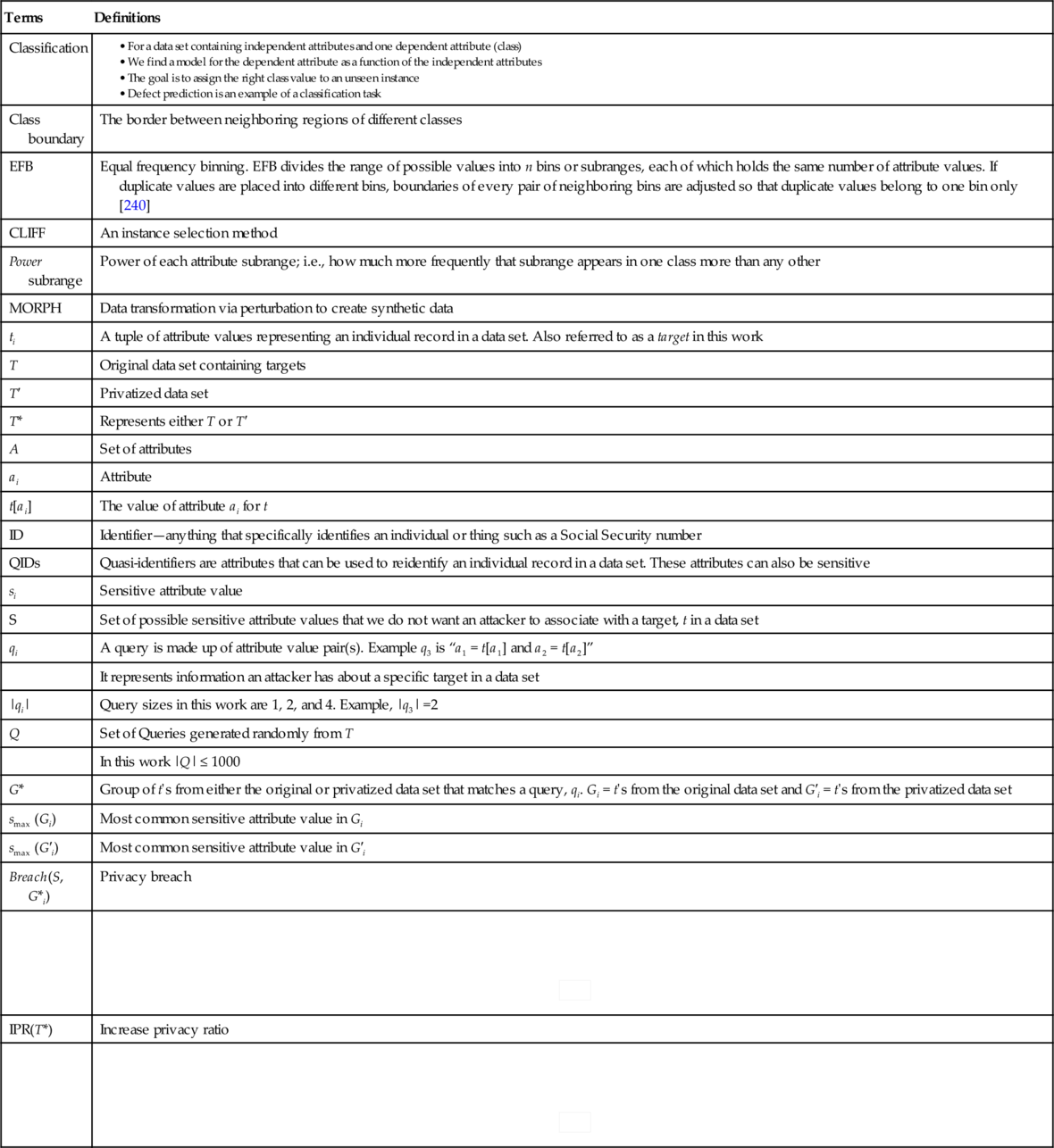
Terms that are related to each other are grouped together.
This study proposes two privatization algorithms. The CLIFF instance pruner finds attribute subranges in the data that are more present in one class versus any other classes. These power subranges are those that drive instances farthest from the class boundaries. If an instance lacks these power subranges then their classification is more ambiguous. CLIFF deletes the instances with the fewest power subranges.
After CLIFF, the MORPH instance mutator perturbs all instance values by a random amount. This amount is selected to create a new instance that is different from the original instance and does not cross class boundaries.
Potentially, CLIFF&MORPH can increase privacy in three ways. First, CLIFF preserves the privacy of the individuals it deletes (these data are no longer available). Second, MORPH increases the privacy of all mutated individuals because their original data is now distorted. Last, to ensure that MORPHed instances are different from instances in the original data set, if a MORPHed instance matches an instance from the original data, it is either MORPHed again until it no longer matches the original or it is removed.
To assess the privacy and utility of CLIFF&MORPH we explore three research questions:
• RQ1: Does CLIFF&MORPH provide better balance between privacy and utility than other state-of-the-art privacy algorithms?
• RQ2: Do different classifiers affect the experimental results?
• RQ3 : Does CLIFF&MORPH perform better than MORPH?
16.6.1 Results and contributions
The experiments of this study show that after applying CLIFF&MORPH, both the efficacy of classification and privacy are increased. Also, combining CLIFF&MORPH improves on prior results. Previously, Peters and Menzies [355] used MORPH and found that, sometimes, the privatized data exhibited worse performance than the original data. In this study, we combine CLIFF&MORPH and show that there is no significant reductions in the classification performance in any of the data sets we study. Note that these are CCDP results where data from many outside companies were combined to learn defect predictors for a local company.
Further, it is well known that pruning before classifying usually saves time [368]. For instance, tomcat, the largest data set used in the study is more than 163 times faster when CLIFF prunes away 90% of the data prior to MORPHing. That is, using this combination of CLIFF&MORPH, we achieve more privacy for effective CCDP in less time.
These results are novel and promising. To the best of our knowledge, this is the first report of a privacy algorithm that increases privacy while preserving inference power. Hence, we believe CLIFF&MORPH is a better option for preserving privacy in a scenario where data is shared for the purpose of CCDP.
16.6.2 Privacy and CCDP
Data sharing across companies exposes the data provider to unwanted risks. Some of these concerns reflect the low quality of our current anonymization technologies. For example, recall when the state of Massachusetts released some health-care data anonymized according to HIPPA regulations [176]. This “anonymized” data was joined to other data (Massachusetts' list of registered voters) and it was possible to identify which health-care data corresponded to specific individuals (e.g., former Massachusetts governor William Weld [412]).
We mentioned earlier that reidentification occurs when an attacker with external information such as a voters' list, can identify an individual from a privatized data set. The data sets used in this study are aggregated at the project level and do not contain personnel or company information. Hence, reidentification of individuals is not explored further in this study.
On the other hand, sensitive attribute disclosure is of great concern with the data used in this study. This is where an individual in a data set can be associated with a sensitive attribute value; e.g., software development time. Such sensitive attribute disclosure can prove problematic. Some of the metrics contained in defect data can be considered as sensitive to the data owners. These can include lines of code (loc) or cyclomatic complexity (max-cc or avg-cc).2 If these software measures are joined to development time, privacy policy may be breached by revealing (say) slow development times.
This section describes how we use CLIFF&MORPH to privatize data sets. As mentioned in Section 16.1, privatization with CLIFF&MORPH starts with removing a certain percentage of the original data. For our experiments we remove 90%, 80%, and 60% of the original data with CLIFF (Section 16.6.3). The remaining data is then MORPHed (Section 16.6.4). The result is a privatized data set with fewer instances, none of which could be found in the original data set. When we perform our CCDP experiments, we combine multiple CLIFFed + MORPHed data sets to create a defect predictor that is used to predict defects in nonprivatized data sets. An example of how CLIFF&MORPH work together is provided in Section 16.6.5.
16.6.3 CLIFF
CLIFF is an instance pruner that assumes tables of training data can be divided into classes. For example, for a table of defect data containing code metrics, different rows might be labeled accordingly (defective or not defective).
CLIFF executes as follows:
• For each column of data, find the power of each attribute subrange; in other words, how much more frequently that subrange appears in one class more than any other.
• In prior work [357], at this point we selected the subrange with the highest power and removed all instances without this subrange. From the remaining instances, those with subranges containing the second highest power were kept while the others were removed. This process continued until at least two instances were left or to the point before there were zero instances left.
• In this work, to control the amount of instances left by CLIFF, we find the product of the powers for each row, then remove the less powerful rows.
The result is a reduced data set with fewer rows. In theory, this reduced data set is less susceptible to privacy breaches.
Algorithm 1: Power is based on BORE [184]. First we assume that the target class is divided into one class as first and the other classes as rest. This makes it easy to find the attribute values that have a high probability of belonging to the current first class using Bayes' theorem. The theorem uses evidence E and a prior probability P(H) for hypothesis H ∈ {first, rest}, to calculate a likelihood (hereafter, like) of the evidence selecting for one class:
This calculation is then normalized to create probabilities:
Jalali et al. [184] found that Equation (16.1) was a poor ranking heuristic for low-frequency evidence. To alleviate this problem, the support measure was introduced. Note that like(first|E) is also a measure of support because it is maximal when a value occurs all the time in every example of one class. Hence, adding the support term is just

To compute the power of a subrange, we first apply equal frequency binning (EFB) to each attribute in the data set. EFB divides the range of possible values into n bins or subranges, each of which holds the same number of attribute values. However, to avoid duplicate values being placed into different bins, boundaries of every pair of neighboring bins are adjusted so that duplicate values should belong to one bin only [240]. For these experiments, we did not optimize the value for n for each data set. We simply used n = 10 bins. In future work we will dynamically set the value of n for a given data set.
Algorithm 1
Finding Subrange Power
1: Power(D, E) {D is the data-set, and E is a set of sub-ranges for a given attribute}
2: Partition(D) ![]() C {Returns data partitioned according to the class label.}
C {Returns data partitioned according to the class label.}
3: PR ← ∅ {Initialize sub-ranges with power for each sub-range in E}
4: for j=0 to # of class values in |C| do
5: first ← Cj
6: rest ← C≠j
7:  {Probability of first data}
8: ![]() {Probability of rest data}
{Probability of rest data}
9: for k=0 to # of sub-ranges in |E| do
10: like(first|Ek) ← number of times Ek appears in first × pfirst
11: like(rest|Ek) ← number of times Ek appears in rest × prest
12: ![]()
13: PR ← powerk
14: end for
15: end for
16: return PR
Next, CLIFF selects p% of the rows in a data set D containing the most powerful subranges. The matrix M holds the result of Power for each attribute, for each class in D. This is used to help select the rows from D to produce D′ within CliffSelection.
The for-loop in lines 3-9 of Algorithm 2 iterates through attributes in D and UniqueRanges is called to find and return the unique subranges for each attribute. Inside that loop, at lines 5-8, a nested for-loop iterates through the unique subranges for a given attribute and Power is called to find the power of each subrange. Last, once the powers are found for each attribute subrange, CliffSelection is called to determine which rows in D will make up the final sample in D':
• Partition D by the class label.
• For each row in each partition, find the product of the power of the subranges in that row.
• For each partition, return the p percent of the partitioned data with the highest power.
An example of how CLIFF is applied to a data set is described in Section 16.6.5.
Algorithm 2
The CLIFF Algorithm
1: CLIFF (D, p) {D is the original data-set, and p is the percentage of data to be returned}
2: M ← ∅ {Initialize sub-range power for each attribute}
3: for i=0 to # of attributes in D do
4: UniqueRanges(Di) ![]() Ri {Returns set of unique sub-ranges for a given attribute}
Ri {Returns set of unique sub-ranges for a given attribute}
5: for j=0 to # of sub-ranges in Ri do
6: Power(D, Ri) ![]() PRj {Returns the sub-ranges with their powers for each class}
PRj {Returns the sub-ranges with their powers for each class}
7: M ← PRj
8: end for
9: end for
10: CliffSelection(D, p, M) ![]() D' {Returns p of the original data}
D' {Returns p of the original data}
11: return D'
16.6.4 MORPH
MORPH is an instance mutator used as a privacy algorithm [355]. It changes the numeric attribute values of each row by replacing these original values with MORPHed values.
The trick to MORPHing data is to keep the new values close enough to the original in order to maintain the utility of the data but far enough to keep the original data private. MORPHed instances are created by applying Equation (16.3) to each attribute value of the instance. MORPH takes care never to change an instance such that it moves across the boundary between the original instance and instances of another class. This boundary is determined by r in Equation (16.3). The smaller r is the closer the boundary is to the original row, and the larger r is the farther away the boundary is to the original row.
Let x ∈ data be the original instance to be changed, y the resulting MORPHed instance, and z ∈ data the nearest unlike neighbor of x, whose class label is different from x's class label. Distance is calculated using the Euclidean distance. The random number r is calculated with the property
where α = 0.15 and β = 0.35. This range of values for r worked previously in our work on MORPH [355].
A simple hashing scheme lets us check if the new instance y is the same as an existing instance (and we keep MORPHing x until it does not hash to the same value as an existing instance). Hence, we can assert that none of the original instances are found in the final data set.
An example of how MORPH is applied to a data set is described in Section 16.6.5.
16.6.5 Example of CLIFF&MORPH
For this example we use the abbreviated version of the ant-1.3 data set shown in Table 16.2a. This data set contains 10 attributes. One dependent attribute (class) and nine independent attributes. Each row is labeled as 1 (containing at least one defect) or 0 (having no defects). The first column holds the row number and each cell contains the original metric values.
Table 16.2
Example of CLIFF&MORPH
| # | wmc | dit | noc | cbo | rfc | lcom | ca | ce | loc | class |
| (a) Partial ant-1.3 defect data | ||||||||||
| 1 | 11 | 4 | 2 | 14 | 42 | 29 | 2 | 12 | 395 | 0 |
| 2 | 14 | 1 | 1 | 8 | 32 | 49 | 4 | 4 | 297 | 1 |
| 3 | 3 | 2 | 0 | 1 | 9 | 0 | 0 | 1 | 58 | 0 |
| 4 | 12 | 3 | 0 | 12 | 37 | 32 | 0 | 12 | 310 | 0 |
| 5 | 6 | 3 | 0 | 4 | 21 | 1 | 0 | 4 | 136 | 0 |
| 6 | 5 | 1 | 5 | 12 | 11 | 8 | 11 | 1 | 59 | 0 |
| 7 | 4 | 2 | 0 | 3 | 16 | 0 | 0 | 3 | 59 | 0 |
| 8 | 14 | 1 | 0 | 24 | 63 | 63 | 20 | 20 | 822 | 1 |
| (b) ant-1.3 after equal frequency binning | ||||||||||
| 1 | (6-14] | [1-4] | [0-5] | (8-24] | (21-63] | (8-63] | (2-20] | (4-20] | (136-822] | 0 |
| 2 | (6-14] | [1-4] | [0-5] | [1-8] | (21-63] | (8-63] | (2-20] | [1-4] | (136-822] | 1 |
| 3 | [3-6] | [1-4] | [0-5] | [1-8] | [9-21] | [0-8] | 0 | [1-4] | [58-136] | 0 |
| 4 | (6-14] | [1-4] | [0-5] | (8-24] | (21-63] | (8-63] | 0 | (4-20] | (136-822] | 0 |
| 5 | [3-6] | [1-4] | [0-5] | [1-8] | [9-21] | [0-8] | 0 | [1-4] | [58-136] | 0 |
| 6 | [3-6] | [1-4] | [0-5] | (8-24] | [9-21] | [0-8] | (2-20] | [1-4] | [58-136] | 0 |
| 7 | [3-6] | [1-4] | [0-5] | [1-8] | [9-21] | [0-8] | 0 | [1-4] | [58-136] | 0 |
| 8 | (6-14] | [1-4] | [0-5] | (8-24] | (21-63] | (8-63] | (2-20] | (4-20] | (136-822] | 1 |
| (c) ant-1.3 power values | ||||||||||
| 1 | 0.13 | 0.56 | 0.60 | 0.28 | 0.13 | 0.13 | 0.28 | 0.17 | 0.28 | 0 |
| 2 | 0.13 | 0.06 | 0.06 | 0.03 | 0.13 | 0.13 | 0.03 | 0.03 | 0.03 | 1 |
| 3 | 0.50 | 0.56 | 0.56 | 0.28 | 0.50 | 0.50 | 0.75 | 0.40 | 0.50 | 0 |
| 4 | 0.13 | 0.56 | 0.56 | 0.28 | 0.13 | 0.13 | 0.75 | 0.17 | 0.28 | 0 |
| 5 | 0.50 | 0.56 | 0.56 | 0.28 | 0.50 | 0.50 | 0.75 | 0.40 | 0.50 | 0 |
| 6 | 0.50 | 0.56 | 0.56 | 0.28 | 0.50 | 0.50 | 0.28 | 0.40 | 0.50 | 0 |
| 7 | 0.50 | 0.56 | 0.56 | 0.28 | 0.50 | 0.50 | 0.75 | 0.40 | 0.50 | 0 |
| 8 | 0.13 | 0.06 | 0.06 | 0.03 | 0.13 | 0.13 | 0.03 | 0.04 | 0.03 | 1 |
| (d) CLIFF result | ||||||||||
| 3 | 3 | 2 | 0 | 1 | 9 | 0 | 0 | 1 | 58 | 0 |
| 8 | 14 | 1 | 0 | 24 | 63 | 63 | 20 | 20 | 822 | 1 |
| (e) MORPH result | ||||||||||
| 3 | 2 | 2 | 0 | 1 | 5 | 5 | 2 | 0 | 1 | 0 |
| 8 | 15 | 1 | 0 | 26 | 67 | 68 | 22 | 21 | 879 | 1 |

(a) Shows the original data and is an abbreviated version of ant-1.3. (b) Data from a binned using EFB. (c) Power values for each subrange in b. (d) CLIFF result. (e) MORPH result.
The bold rows show what rows have most power for predicting for class “1” or class “0”.
The result of applying CLIFF&MORPH is shown in Table 16.2e. To get to that point, first the original data is binned using EFB. The result of this is shown in Table 16.2b. For example the attribute values of wmc are replaced by two subranges of values ([3-6] and (6-14]). Here all values from 3 to 6 inclusive are placed in the first subrange and all values between 6 and 14 (not including 6) are placed in the last subrange.
Following this, each subrange is the ranked according to Equation (16.2). To find the power of each subrange, we first divide the data into first and rest. For this example, let us say that all the rows with the 0 class label are first while the others are rest. Figure 16.4 shows an example of finding the power of (6-14] for attribute wmc, and Table 16.2c shows the power values for all the subranges of Table 16.2b.

Next, the power of each row is calculated by finding the product of the subrange powers of each row. In this example the row with the highest power for each class is selected. In this case that is row 3 for the 0 class label and row 8 for the 1 class label. This result is shown in Table 16.2d.
Finally, we MORPH this result according to Equation (16.3) to obtain the result in Table 16.2e.
16.6.6 Evaluation metrics
This section assesses the privacy and utility offered by CLIFF&MORPH.
16.6.7 Evaluating utility via classification
We say that the classification performance of a privatized data set is adequate if it performs no worse than the baseline computed from the original data set defined as follows:
For data-sets in T, T1,…, T|T|, performance data is collected when a defect model is learned from the All − Ti, then applied to Ti.
Table 16.3 defines performance measures used in this work to assess defect predictors. It also includes a new measure used in this work called the g-measure.
Table 16.3
Some Popular Measures Used in Software Defect Prediction Work
| Actual | |||
| Yes | No | ||
| Predicted | Yes | TP | FP |
| No | FN | TN | |
| Recall (pd) | |||
| pf | |||
| g-Measure | |||

• Recall, or pd, measures how many of the target (defective) instances are found. The higher the pd, the fewer the false negative results;
• Probability of false alarm, or pf, measures how many of the instances that triggered the detector actually did not contained the target (defective) concept. Like pd, the highest pf is 100% however its desired result is 0%;
• g-measure (harmonic mean of pd and 1 – pf): In this work, we report on the g-measure. The 1 – pf represents specificity (not predicting instances without defects as defective). Specificity (1 – pf) is used together with pd to form the G-mean2 measure seen in Jiang et al. [186]. It is the geometric mean of the pds for both the majority and the minority class. In our case, we use these to form the g-measure which is the harmonic mean of pd and 1 – pf.
Other measures such as accuracy, precision, and f-measure were not used as they are poor indicators of performance for data where the target class is rare (in our case, the defective instances). This is based on a study done by Menzies et al. [303] that shows that when data sets contain a low percentage of defects, precision can be unstable. If we look at the data sets in Table 16.4, we see that the percentage of defects are low in most cases.

16.6.8 Evaluating privatization
In Section 16.5.1, we talked about the different privacy measures used in different studies. The existence of multiple privacy measures raises the question, “How do the different privacy measures compare with each other?” We will investigate this issue in future work. However, here we use IPR because it is based on work done by Brickell and Shmatikov [57].
Privacy is not a binary step function where something is either 100% private or 100% disclosed. Rather it is a probabilistic process where we strive to decrease the likelihood that an attacker can uncover something that they should not know. The rest of this section defines privacy using a probabilistic increased privacy ratio, or IPR, of privatized data sets.
16.6.8.1 Defining privacy
To investigate how well the original defect data is privatized, we assume the role of an attacker armed with some background knowledge from the original data set and also supplied with the private data set. In order to keep the privatized data set truthful, Brickell and Shmatikov [57] kept the sensitive attribute values as is and privatized only the QIDs. However in this work, in addition to privatizing the QIDs with CLIFF&MORPH, we apply EFB to the sensitive attribute to create 10 subranges of values to easily report on the privacy level of the privatized data set.
We propose the following privacy metric based on the adversarial accuracy gain, Aacc from the work of Brickell and Shamtikov [57]. According to the authors definition of Aacc, it quantifies an attacker's ability to predict the sensitive attribute value of a target t. The attacker accomplishes this by guessing the most common sensitive attribute value in 〈t〉, (a QID group).
Specifically, Aacc measures the increase in the attacker's accuracy after he observes a privatized data set and compares it to the baseline from a trivially privatized data set which offers perfect privacy by removing either all sensitive attribute values or all the other QIDs.
Recall that we assume that the attacker has access to a privatized version (T′) of an original data set (T), and knowledge of nonsensitive QID values for a specific target in T. We refer to the latter as a query. For our experiments we randomly generate up to 1000 of these queries, |Q| ≤ 1000 (Section 16.6.12 describes how queries are generated).
For each query, q in a set Q = {q1,…, q|Q|}, G*i is a group of rows from any data set that matches qi. Hence, let Gi be the group from the original data set and G′i be the group from the privatized data set that matches qi. Next, for every sensitive attribute subrange in the set S = {s1,…, s|S|}, we denote the idea of the most common sensitive attribute value as smax(G*i).
Now, we define a breach of privacy as follows:
Therefore, the privacy level of the privatized data set is
IPR(T*) stands for increased privacy ratio and has some similarity to Aacc of Brickell and Shamtikov [57], where IPR(T*) measures the attacker's ability to cause privacy breaches after observing the privatized data set T′ compared to a baseline of the original data set T. To be more precise, IPR(T*) measures the percent of total queries that did not cause a privacy Breach.
We baseline our work against the original data set (our worst-case scenario) which offers no privacy and therefore its IPR(T) = 0. In our case, to have perfect privacy (our best-case scenario) we create a privatized data set by simply removing the sensitive attribute values. This will leave us with IPR(T′) = 1.
16.6.9 Experiments
16.6.9.1 Data
In order to assist replication, our data comes from the online PROMISE data repository [300]. Table 16.5 describes the attributes of these data sets and Table 16.4 shows other details.
Table 16.5
The C-K Metrics of the Data Sets Used in this Work (see Table 16.4)
| Attributes | Symbols | Description |
| Average method complexity | amc | For example, number of JAVA byte codes |
| Average McCabe | avg_cc | Average McCabe's cyclomatic complexity seen in class |
| Afferent couplings | ca | How many other classes use the specific class |
| Cohesion amongst classes | cam | Summation of number of different types of method parameters in every method divided by a multiplication of number of different method parameter types in whole class and number of methods |
| Coupling between methods | cbm | Total number of new/redefined methods to which all the inherited methods are coupled |
| Coupling between objects | cbo | Increased when the methods of one class access services of another |
| Efferent couplings | ce | How many other classes is used by the specific class |
| Data access | dam | Ratio of the number of private (protected) attributes to the total number of attributes |
| Depth of inheritance tree | dit | Provides the position of the class in the inheritance tree |
| Inheritance coupling | ic | Number of parent classes to which a given class is coupled (includes counts of methods and variables inherited) |
| Lack of cohesion in methods | lcom | Number of pairs of methods that do not share a reference to an instance variable |
| Another lack of cohesion measure | locm3 | If m, a are the number of methods, attributes in a class number and μ(a) is the number of methods accessing an attribute, then  |
| Lines of code | loc | Measures the volume of code |
| Maximum McCabe | max_cc | Maximum McCabe's cyclomatic complexity seen in class |
| Functional abstraction | mfa | Number of methods inherited by a class plus number of methods accessible by member methods of the class |
| Aggregation | moa | Count of the number of data declarations (class fields) whose types are user-defined classes |
| Number of children | noc | Measures the number of immediate descendants of the class |
| Number of public methods | npm | Counts all the methods in a class that are declared as public. The metric is known also as class interface size (CIS) |
| Response for a class | rfc | Number of methods invoked in response to a message to the object |
| Weighted methods per class | wmc | The number of methods in the class (assuming unity weights for all methods) |
| Defects | defects | Number of defects per class, seen in postrelease bug-tracking systems |
The last row is the dependent variable. Jureczko and Madeyski [198] provide more information on these metrics.
16.6.10 Design
From our experiments, the goal is to determine whether we can have effective defect prediction from shared data while preserving privacy. To test the shared data scenario, we do CCDP experiments for all the data sets of Table 16.4 in their original state and after they have been privatized. When experimenting with the original data, from the 10 data sets used, one is used as a test set while a defect predictor was made from All the data in the other nine data sets. This process is repeated for each data set. The same process is followed when the data sets are privatized. Each of the nine data sets used to create a defect predictor are first privatized, then combined into All. The test set is not privatized.
In a separate experiment to test how private the data sets are after the privatization algorithms are applied, we model an attacker's background knowledge with queries (see Section 16.6.12). These queries are applied to both the original and privatized data sets. The IPRs for each privatized data set are then calculated (see Section 16.6.8).
16.6.11 Defect predictors
To analyze the utility of CLIFF&MORPH, we perform CCDP experiments with three classification techniques implemented in WEKA [156]. These are Naive Bayes (NB) [252], support vector machines (SVMs) [360], and neural networks (NN) [33]. The default values for these classifiers in WEKA are used in our experiments.
These three classification techniques have been widely used for defect prediction [157, 249, 294]. Lewis [252] describes NB as a classifier based on Bayes' rule. It is a statistical-based learning scheme that assumes attributes are equally important and statistically independent. To classify an unknown instance, NB chooses the class with the maximum likelihood of containing the evidence in the test case. SVMs seek to minimize misclassification errors by selecting a boundary or hyperplane that leaves the maximum margin between the two classes, where the margin is defined as the sum of the distances of the hyperplane from the closest point of the two classes [350]. According to Lessmann et al. [249], NNs depict a network structure that defines a concatenation of weighting, aggregation, and thresholding functions that are applied to a software module's attributes to obtain an approximation of its posterior probability of being fault prone.
16.6.12 Query generator
A query generator is used to provide a sample of attacks on the data. Before discussing the query generator, a few details must be established. First, to maintain some “truthfulness” to the data, a selected sensitive attribute and the class attribute are not used as part of query generation. Here we are assuming that the only information an attacker could have is information about the nonsensitive QIDs in the data set. As a result these attribute values (sensitive and class) are unchanged in the privatized data set.
To illustrate the application of the query generator, we use Table 16.2a and b. First EFB is applied to the original data in Table 16.2a to create the subranges shown in Table 16.2b. Next, to create a query, we proceed as follows:
1. Given a query size (measured as the number of {attribute subrange} pairs; for this example we use a query size of 1);
2. Given the set of attributes A = (wmc, dit, noc, cbo, rfc, lcom, ca, ce) and all their possible subranges;
3. Randomly select an attribute from A, e.g., wmc with two possible subranges (6-14] and [0-6];
4. Randomly select a subrange from all possible subranges of wmc, e.g., (6-14].
In the end the query we generate is, wmc = (6-14]. Table 16.6, shows more examples of queries, their sizes, and the number and rows they match from the data set.
Table 16.6
Example: Queries, Query Sizes and the Number of Rows that Match the Queries, |G|
| Query | Size | |G| | Row# |
| cbo = (8-24] | 1 | 4 | 1,4,6,8 |
| cbo = (8-24] and wmc = (6-14] | 2 | 3 | 1,4,8 |
| cbo = (8-24] and wmc = (6-14] and noc = [0-5] and ca = 0 | 4 | 1 | 4 |

Table 16.2b is used for this example.
For each query size, we generate up to 1000 queries because it is not practical to test every possible query. With these data sets the number of possible queries with arity 4 and no repeats is 38,760,000.3
Each query must also satisfy the following sanity checks:
• It must not include attribute value pairs from either the designated sensitive attribute or the class attribute.
• It must return at least two instances after a search of the original data set.
• It must not be the same as another query no matter the order of the individual {attribute subrange} pairs in the query.
16.6.13 Benchmark privacy algorithms
In order to benchmark our approach, we compare it against data swapping and k-anonymity. Data swapping is a standard perturbation technique used for privacy [138, 413, 457]. This is a permutation approach that disassociates the relationship between a nonsensitive QID and a numerical sensitive attribute. In our implementation of data swapping, for each QID a certain percent of the values are swapped with any other value in that QID. For our experiments, these percentages are 10%, 20%, and 40%.
An example of k-anonymity is shown in Figure 16.3. Our implementation follows the Datafly algorithm [411] for k-anonymity. The core Datafly algorithm starts with the input of a set of QIDs, k, and a generalization hierarchy. An example of a hierarchy is shown in the tree below using the values of wmc from Table 16.2a. Values at the leaves are generalized by replacing them with the subranges [3-6] or (6-14]. These in turn can be replaced by [3-14]. Or the leaf values can be suppressed by replacing them with a symbol such as the stars at the top of the tree.

Datafly then replaces values in the QIDs according to the hierarchy. This generalization continues until there are k or fewer distinct instances. These instances are suppressed.
16.6.14 Experimental evaluation
This section presents the results of our experiments. Before going forward, Table 16.7 shows the notation and meaning of the algorithms used in this work.
Table 16.7
Algorithm Characteristics
| Algorithms | Symbol | Meaning |
| MORPHed | m | Data privatized by MORPH only |
| MORPHedX | mX: m10, m20, m40 | X represents the percentage of the original data that remains after CLIFF is applied and m indicates that the remaining data is then MORPHed. These are collectively referred to as CLIFF&MORPH algorithms |
| swappedX | sX: s10, s20, s40 | X represents the percentage of the original data swapped |
| X-anonymity | kX: k2, k4 | X represents the size of the QID group, where each member of the group is indistinguishable from k − 1 others in the group |
RQ1: Does CLIFF&MORPH provide better balance between privacy and utility than other state-of-the-art privacy algorithms?
To see whether CLIFF&MORPH offers a better balance between privacy and utility, we privatized the original data sets shown in Table 16.4 with data swapping, k-anonymity, and CLIFF&MORPH. Then, the IPR and g-measures are calculated for each privatized data set. The experimental results are displayed in Figure 16.5. For each chart, we plot IPR on the x-axis and g-measures on the y-axis. The g-measures are based on the NB and the IPR based on queries of size 1. There is not enough space here to repeat Figure 16.5 for each query size and each classifier used in this work (a total of nine figures). Instead, we present IPR results for query sizes 2 and 4 in Table 16.8, and g-measures for NB, SVM, and NN in Tables 16.9–16.11, respectively.

Table 16.8
The IPR for Query Sizes 2 and 4
| Data | m | m10 | m20 | m40 | s10 | s20 | s40 | k2 | k4 |
| Query size = 2 | |||||||||
| ant-1.3 | 77.1 | 97.3 | 95.9 | 91.9 | 60.2 | 67.6 | 78.6 | 98.4 | 99.9 |
| arc | 75.4 | 99.4 | 98.3 | 96.8 | 60.7 | 64.7 | 79.0 | 94.0 | 99.2 |
| camel-1.0 | 80.3 | 95.6 | 94.1 | 93.9 | 62.3 | 68.2 | 78.7 | 89.9 | 94.7 |
| poi-1.5 | 76.2 | 97.9 | 97.1 | 94.6 | 60.5 | 66.9 | 74.1 | 90.7 | 95.3 |
| redaktor | 75.3 | 94.9 | 93.7 | 90.8 | 61.3 | 64.2 | 76.2 | 89.3 | 97.6 |
| skarbonka | 77.5 | 99.7 | 97.9 | 96.1 | 57.5 | 65.0 | 76.6 | 98.8 | 100.0 |
| tomcat | 79.6 | 98.2 | 96.0 | 90.6 | 64.0 | 69.6 | 73.9 | 92.9 | 96.6 |
| velocity-1.4 | 76.6 | 96.0 | 94.6 | 90.5 | 60.1 | 65.8 | 75.7 | 92.9 | 95.4 |
| xalan-2.4 | 79.6 | 96.5 | 93.9 | 91.8 | 63.6 | 67.8 | 76.3 | 93.4 | 97.0 |
| xerces-1.2 | 76.7 | 100.0 | 99.2 | 96.9 | 58.3 | 64.1 | 72.6 | 89.6 | 95.1 |
| Median | 76.9 | 97.6 | 96.0 | 92.9 | 60.6 | 66.4 | 76.3 | 92.9 | 96.8 |
| Query size = 4 | |||||||||
| ant-1.3 | 78.6 | 97.5 | 97.0 | 95.4 | 62.2 | 68.5 | 78.3 | 99.6 | 99.6 |
| arc | 78.0 | 99.5 | 98.6 | 98.2 | 59.3 | 69.2 | 77.7 | 99.2 | 100.0 |
| camel-1.0 | 75.0 | 81.1 | 80.4 | 80.0 | 57.9 | 67.3 | 72.8 | 80.0 | 80.8 |
| poi-1.5 | 78.0 | 99.8 | 99.5 | 98.9 | 60.8 | 70.6 | 77.9 | 97.5 | 98.4 |
| redaktor | 81.6 | 98.8 | 97.6 | 95.9 | 60.2 | 68.0 | 77.5 | 95.8 | 100.0 |
| skarbonka | 61.5 | 100.0 | 100.0 | 98.9 | 56.2 | 59.0 | 64.2 | 100.0 | 100.0 |
| tomcat | 84.3 | 99.7 | 99.5 | 98.8 | 61.3 | 72.3 | 85.0 | 99.1 | 99.8 |
| velocity-1.4 | 77.8 | 100.0 | 98.7 | 98.1 | 59.8 | 67.8 | 77.7 | 99.1 | 99.5 |
| xalan-2.4 | 81.1 | 99.9 | 99.1 | 98.2 | 60.4 | 69.7 | 80.0 | 99.2 | 100.0 |
| xerces-1.2 | 78.3 | 100.0 | 100.0 | 100.0 | 59.8 | 65.5 | 77.6 | 99.0 | 99.5 |
| Median | 78.2 | 99.8 | 98.9 | 98.2 | 60.0 | 68.3 | 77.7 | 99.1 | 99.7 |
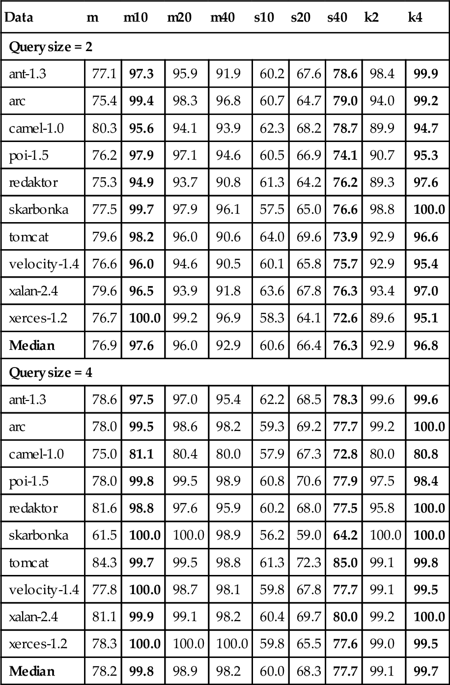
(From [356].)
The numbers in bold are the highest for the different types of privacy algorithms.
Table 16.9
The Cross-Company Experiment for 10 Data Sets with Naive Bayes: The pds, pfs, and g-Measures are Shown with the g-Measures Shown in Bold
| NB | orig | m | m10 | m20 | m40 | s10 | s20 | s40 | k2 | k4 | |
| ant1.3 | g | 26 | 26 | 42 | 59 | 68 | 26 | 26 | 18 | 18 | 18 |
| pd | 15 | 15 | 95 | 85 | 90 | 15 | 15 | 10 | 10 | 10 | |
| pf | 5 | 7 | 73 | 55 | 46 | 5 | 5 | 5 | 7 | 7 | |
| arc | g | 36 | 31 | 59 | 64 | 66 | 36 | 31 | 36 | 31 | 31 |
| pd | 22 | 19 | 81 | 67 | 59 | 22 | 19 | 22 | 19 | 19 | |
| pf | 5 | 5 | 54 | 38 | 26 | 5 | 5 | 5 | 5 | 5 | |
| camel1.0 | g | 62 | 62 | 51 | 59 | 62 | 62 | 47 | 47 | 55 | 55 |
| pd | 46 | 46 | 92 | 77 | 62 | 46 | 31 | 31 | 38 | 38 | |
| pf | 5 | 5 | 64 | 52 | 38 | 3 | 4 | 4 | 4 | 4 | |
| poi1.5 | g | 24 | 23 | 52 | 61 | 64 | 24 | 17 | 16 | 20 | 19 |
| pd | 13 | 13 | 84 | 78 | 54 | 13 | 9 | 9 | 11 | 11 | |
| pf | 4 | 4 | 63 | 50 | 22 | 4 | 3 | 3 | 4 | 4 | |
| redaktor | g | 14 | 14 | 20 | 34 | 54 | 7 | 14 | 0 | 20 | 14 |
| pd | 7 | 7 | 96 | 89 | 78 | 4 | 7 | 0 | 11 | 7 | |
| pf | 7 | 5 | 89 | 79 | 59 | 7 | 7 | 3 | 7 | 6 | |
| skarbonka | g | 0 | 0 | 70 | 72 | 70 | 0 | 0 | 0 | 0 | 0 |
| pd | 0 | 0 | 89 | 89 | 78 | 0 | 0 | 0 | 0 | 0 | |
| pf | 8 | 8 | 42 | 39 | 36 | 8 | 3 | 3 | 3 | 3 | |
| tomcat | g | 69 | 67 | 54 | 64 | 71 | 67 | 62 | 63 | 52 | 48 |
| pd | 57 | 55 | 92 | 88 | 81 | 55 | 48 | 48 | 36 | 32 | |
| pf | 12 | 12 | 62 | 50 | 36 | 12 | 11 | 10 | 9 | 8 | |
| velocity1.4 | g | 11 | 10 | 31 | 35 | 44 | 10 | 10 | 9 | 9 | 9 |
| pd | 6 | 5 | 64 | 41 | 35 | 5 | 5 | 5 | 5 | 5 | |
| pf | 12 | 12 | 80 | 69 | 41 | 8 | 8 | 8 | 10 | 10 | |
| xalan2.4 | g | 60 | 60 | 41 | 51 | 55 | 58 | 56 | 58 | 58 | 54 |
| pd | 49 | 48 | 92 | 89 | 88 | 47 | 44 | 45 | 47 | 42 | |
| pf | 24 | 22 | 74 | 64 | 60 | 23 | 22 | 20 | 24 | 23 | |
| xerces1.2 | g | 34 | 34 | 40 | 42 | 44 | 30 | 31 | 30 | 31 | 29 |
| pd | 21 | 21 | 51 | 42 | 34 | 18 | 18 | 18 | 18 | 17 | |
| pf | 9 | 9 | 67 | 59 | 36 | 9 | 8 | 10 | 7 | 7 | |
| Median (g) | 30 | 28 | 47 | 59 | 63 | 28 | 28 | 24 | 25 | 24 |

(From 356].)
Table 16.10
The Cross-Company Experiment for 10 Data Sets with Support Vector Machines: The pds, pfs, and g-Measures are Shown with the g-Measures Shown in Bold
| SVM | orig | m | m10 | m20 | m40 | s10 | s20 | s40 | k2 | k4 | |
| ant1.3 | g | 0 | 0 | 62 | 75 | 75 | 0 | 0 | 0 | 0 | 0 |
| pd | 0 | 0 | 90 | 70 | 70 | 0 | 0 | 0 | 0 | 0 | |
| pf | 0 | 0 | 52 | 20 | 18 | 0 | 0 | 0 | 0 | 0 | |
| arc | g | 0 | 0 | 67 | 59 | 56 | 0 | 0 | 0 | 0 | 0 |
| pd | 0 | 0 | 70 | 44 | 41 | 0 | 0 | 0 | 0 | 0 | |
| pf | 0 | 0 | 36 | 14 | 9 | 0 | 0 | 0 | 0 | 0 | |
| camel1.0 | g | 0 | 0 | 70 | 71 | 67 | 0 | 0 | 0 | 0 | 0 |
| pd | 0 | 0 | 85 | 62 | 54 | 0 | 0 | 0 | 0 | 0 | |
| pf | 0 | 0 | 41 | 16 | 13 | 0 | 0 | 0 | 0 | 0 | |
| poi1.5 | g | 0 | 0 | 54 | 25 | 30 | 0 | 0 | 0 | 0 | 0 |
| pd | 0 | 0 | 41 | 14 | 18 | 0 | 0 | 0 | 0 | 0 | |
| pf | 0 | 0 | 20 | 2 | 4 | 0 | 0 | 0 | 0 | 0 | |
| redaktor | g | 0 | 0 | 40 | 50 | 55 | 0 | 0 | 0 | 0 | 0 |
| pd | 0 | 0 | 63 | 59 | 56 | 0 | 0 | 0 | 0 | 0 | |
| pf | 0 | 0 | 70 | 56 | 46 | 0 | 0 | 0 | 0 | 0 | |
| skarbonka | g | 0 | 0 | 68 | 48 | 35 | 0 | 0 | 0 | 0 | 0 |
| pd | 0 | 0 | 67 | 33 | 22 | 0 | 0 | 0 | 0 | 0 | |
| pf | 0 | 0 | 31 | 14 | 14 | 0 | 0 | 0 | 0 | 0 | |
| tomcat | g | 0 | 0 | 60 | 73 | 65 | 0 | 0 | 0 | 0 | 5 |
| pd | 0 | 0 | 90 | 65 | 51 | 0 | 0 | 0 | 0 | 3 | |
| pf | 0 | 0 | 54 | 16 | 9 | 0 | 0 | 0 | 0 | 0 | |
| velocity1.4 | g | 0 | 0 | 43 | 27 | 18 | 0 | 0 | 0 | 0 | 0 |
| pd | 0 | 0 | 44 | 16 | 10 | 0 | 0 | 0 | 0 | 0 | |
| pf | 0 | 0 | 57 | 16 | 10 | 0 | 0 | 0 | 0 | 0 | |
| xalan2.4 | g | 0 | 0 | 66 | 61 | 62 | 0 | 0 | 0 | 0 | 24 |
| pd | 0 | 0 | 70 | 56 | 63 | 0 | 0 | 0 | 0 | 14 | |
| pf | 0 | 0 | 37 | 34 | 38 | 0 | 0 | 0 | 0 | 2 | |
| xerces1.2 | g | 0 | 0 | 46 | 48 | 42 | 0 | 0 | 0 | 0 | 0 |
| pd | 0 | 0 | 45 | 39 | 28 | 0 | 0 | 0 | 0 | 0 | |
| pf | 0 | 0 | 52 | 38 | 14 | 0 | 0 | 0 | 0 | 0 | |
| Median (g) | 0 | 0 | 61 | 54 | 55 | 0 | 0 | 0 | 0 | 0 |

(From [356].)
Table 16.11
The Cross-Company Experiment for 10 Data Sets with Neural Networks: The pds, pfs, and g-Measures are Shown with the g-Measures Shown in Bold
| NN | orig | m | m10 | m20 | m40 | s10 | s20 | s40 | k2 | k4 | |
| ant1.3 | g | 38 | 32 | 59 | 56 | 62 | 38 | 51 | 44 | 32 | 0 |
| pd | 25 | 20 | 70 | 65 | 65 | 25 | 35 | 30 | 20 | 0 | |
| pf | 17 | 18 | 50 | 51 | 41 | 20 | 7 | 15 | 20 | 7 | |
| arc | g | 57 | 19 | 60 | 60 | 63 | 43 | 42 | 47 | 68 | 0 |
| pd | 44 | 11 | 59 | 59 | 74 | 30 | 30 | 33 | 59 | 0 | |
| pf | 22 | 22 | 40 | 40 | 45 | 20 | 26 | 20 | 20 | 7 | |
| camel1.0 | g | 45 | 57 | 65 | 59 | 52 | 52 | 51 | 58 | 44 | 0 |
| pd | 31 | 46 | 69 | 62 | 46 | 38 | 38 | 46 | 31 | 0 | |
| pf | 19 | 25 | 38 | 43 | 41 | 22 | 24 | 21 | 24 | 6 | |
| poi1.5 | g | 37 | 20 | 45 | 49 | 53 | 33 | 18 | 19 | 42 | 7 |
| pd | 23 | 11 | 31 | 36 | 40 | 21 | 10 | 11 | 29 | 4 | |
| pf | 16 | 16 | 20 | 25 | 25 | 10 | 9 | 8 | 23 | 6 | |
| redaktor | g | 43 | 39 | 56 | 63 | 51 | 29 | 48 | 20 | 67 | 14 |
| pd | 30 | 26 | 74 | 78 | 70 | 19 | 33 | 11 | 59 | 7 | |
| pf | 23 | 23 | 54 | 48 | 60 | 38 | 17 | 17 | 24 | 1 | |
| skarbonka | g | 20 | 33 | 46 | 47 | 63 | 0 | 20 | 20 | 20 | 0 |
| pd | 11 | 22 | 44 | 44 | 56 | 0 | 11 | 11 | 11 | 0 | |
| pf | 19 | 36 | 53 | 50 | 28 | 14 | 11 | 8 | 11 | 0 | |
| tomcat | g | 39 | 38 | 58 | 69 | 68 | 44 | 42 | 46 | 41 | 3 |
| pd | 26 | 25 | 52 | 73 | 68 | 30 | 29 | 32 | 29 | 1 | |
| pf | 20 | 20 | 34 | 34 | 31 | 20 | 18 | 19 | 25 | 8 | |
| velocity1.4 | g | 14 | 15 | 35 | 35 | 37 | 9 | 13 | 15 | 19 | 5 |
| pd | 7 | 8 | 34 | 37 | 29 | 5 | 7 | 8 | 11 | 3 | |
| pf | 4 | 12 | 63 | 67 | 47 | 20 | 4 | 10 | 14 | 0 | |
| xalan2.4 | g | 41 | 44 | 58 | 57 | 62 | 35 | 35 | 39 | 36 | 13 |
| pd | 27 | 30 | 64 | 59 | 65 | 22 | 22 | 25 | 23 | 7 | |
| pf | 17 | 20 | 46 | 46 | 41 | 13 | 13 | 17 | 18 | 11 | |
| xerces1.2 | g | 18 | 28 | 52 | 47 | 45 | 13 | 26 | 13 | 18 | 16 |
| pd | 10 | 17 | 56 | 35 | 32 | 7 | 15 | 7 | 10 | 8 | |
| pf | 9 | 11 | 51 | 31 | 24 | 11 | 11 | 11 | 14 | 6 | |
| Median (g) | 39 | 33 | 57 | 56 | 57 | 34 | 39 | 29 | 38 | 4 |

In Figure 16.5, the horizontal and vertical lines show the CCDP g-measures of the original data set and IPR= 80%, respectively. To answer RQ1, we say that the privatized data sets appearing to the right and above these lines, are private enough (IPR over 80%) and perform adequately (as good or better than the nonprivatized data). In other words this region corresponds to data that provide the best balance between privacy and utility.
Note that for most cases, ![]() , the CLIFF&MORPH algorithms (m10, m20, and m40) fall to the right and above these lines. We expect this result for IPRs; however, one may question why the g-measures are higher than those of the original data set in those seven cases. This is due to instance selection done by CLIFF. Research has shown that instance selection can produce comparable or improved classification results [58, 357]. This makes CLIFF a perfect compliment to MORPH. Other studies on instance selection are included in the surveys [29, 30, 211, 346].
, the CLIFF&MORPH algorithms (m10, m20, and m40) fall to the right and above these lines. We expect this result for IPRs; however, one may question why the g-measures are higher than those of the original data set in those seven cases. This is due to instance selection done by CLIFF. Research has shown that instance selection can produce comparable or improved classification results [58, 357]. This makes CLIFF a perfect compliment to MORPH. Other studies on instance selection are included in the surveys [29, 30, 211, 346].
Of the three remaining data sets (camel-1.0, tomcat, and xalan-2.4), all offer IPRs above the 80% baseline; however, their g-measures are either as good as those of the original data set or worse. This is particularly true in the case of xalan-2.4. We see this as an issue concerning the structure of the data set rather than the CLIFF&MORPH algorithms themselves, considering that it performs well for most of the privatized data sets used in this study.
Equally important is the fact that, generally, the data swapping algorithms are less private than the CLIFF&MORPH algorithms and k-anonymity. This effect is seen clearly in Figure 16.5, where all 10 data sets show the best IPRs belonging to the CLIFF&MORPH algorithms and k-anonymity; while the utility of data swapping and k-anonymity are generally as good as or worse than the nonprivatized data set.
This summary of results also holds true when measuring IPRs for query sizes 2 and 4 (Table 16.8), and g-measures for SVM (Table 16.10) and NN (Table 16.11).
So, to answer RQ1, at least for the defect data sets used in this study and the baselines used, CLIFF&MORPH generally provides a better balance between privacy and utility than data swapping and k-anonymity.
RQ2: Do different classifiers affect the experimental results?
Looking at the raw results from Tables 16.9–16.11, the SVM results shown in Table 16.10 stand out for CLIFF&MORPH and the other privacy algorithms. Here, in all cases CLIFF&MORPH has better g-measures, while in ![]() cases, only CLIFF&MORPH has g-measures above zero. The privacy algorithms for NB and the NN generally show better g-measure results than SVM.
cases, only CLIFF&MORPH has g-measures above zero. The privacy algorithms for NB and the NN generally show better g-measure results than SVM.
For a substantial comparison between classifiers we use the Mann-Whitney U test [281] at 95% confidence for the g-measures over all data sets. The results show that there is no significant difference in the performance of NB and NN. However when g-measures from SVM are compared to those of NB and NN, it performs significantly worse. Therefore, to answer RQ2, although the results show that the NB and NN classifiers perform better than SVM, the g-measures show that the CLIFF&MORPH algorithms have the best performance for all three classifiers used in this study. Therefore, based on this result for these different types of classifiers we conclude that the performance of CLIFF&MORPH is not dependent on the type of classifier used.
RQ3: Does CLIFF&MORPH perform better than MORPH?
Previous work by Peters and Menzies [355], showed that a data set privatized by MORPH offered at least four times more privacy than the original data set and comparable utility results. In this work we enhance the performance of the MORPH algorithm by first applying the instance selector CLIFF to the original data set.
All results in this study indicate that CLIFF&MORPH performs better than just MORPH. This is because as CLIFF removes the instances with the fewest power subranges, it is getting rid of those instances that may cause ambiguous classification. This improves utility. An exceptional example of this can be seen in Figure 16.5 with skarbonka. When NB is use to create the defect predictor, we see much higher g-measures for the CLIFF&MORPH algorithms (between 60% and 80%), while the MORPH algorithm has a 0% g-measure. This general trend of the CLIFF&MORPH algorithms having better utility than the MORPH algorithm can also be seen in Figure 16.5 for ant-1.3, arc, poi-1.5, redaktor, velocity-1.4, and xerces-1.2. Additionally, Tables 16.10, 16.11 confirm these results with both SVM and NN having greater median g-measures for the CLIFF&MORPH algorithms than for the MORPH algorithm. The best performance is shown with SVM, where MORPH has a 0% median g-measure and m10 has a median 61% g-measure.
Privacy is improved because we are first removing 90%, 80%, and 60% of the original data, then MORPHing the remaining instances. The removed instances are guaranteed 100% protection due to their absence. By then, applying MORPH to the remaining instances, we have (in all cases) IPRs for the CLIFF&MORPH algorithms that are private enough (>80%) and greater than those for MORPH, which in most cases are not >80%. These results are shown in Figure 16.5 and Table 16.8.
16.6.15 Discussion
As with any empirical study, biases can affect the final results. Therefore any conclusions made from this work must be considered with the following issues in mind:
1. Sampling bias threatens any classification experiment; i.e., what matters there may not be true here. For example, the data sets used here come from the PROMISE repository and were supplied by one individual. The best we can do is define our methods and publicize our data so that other researchers can try to repeat our results and, perhaps, point out a previously unknown bias in our analysis. Hopefully, other researchers will emulate our methods in order to repeat, refute, or improve our results.
2. Learner bias: Another source of bias in this study are the learners used for the defect prediction studies. Classification is a large and active field and any single study can only use a small subset of the known classification algorithms. In this work, only results for NB, SVMs, and NN are published.
3. Evaluation bias: This chapter has focused on background knowledge specific to the original data sets without regard for other types of background knowledge, which cannot be captured by the queries used in this study. For instance, correlation knowledge and knowledge about knowing information about related files. This is a subject for future work.
4. Other evaluation bias: The utility of a privatized data set can be measured semantically (where the workload is unknown) or empirically (known workload, e.g., classification or aggregate query answering). In this work, we measure utility empirically for defect prediction.
5. Comparison bias: There are many anonymization algorithms and it would be difficult to compare the performance of CLIFF&MORPH against them all. This paper compares our approach against privatization methods that are known not to damage classification; this is why we used the data swapping (also used by Taneja et al. [413]). We also used k-anonymity [411], a widely used privacy algorithm.
16.6.16 Related work: privacy in SE
Research on privacy in SE has focused on software testing and debugging [63, 67, 79, 413], and defect prediction [355, 356]. Work published by Castro et al. [67] sought to provide a solution to the problem of software vendors who need to include sensitive user information in error reports in order to reproduce a bug. To protect sensitive user information, Castro et al. [67] used symbolic execution along the path followed by a failed execution to compute path conditions. Their goal was to compute new input values unrelated to the original input. These new input values satisfied the path conditions required to make the software follow the same execution path until it failed.
As a follow-up to the Castro et al. [67] paper, Clause and Orso [79] presented an algorithm that anonymized input sent from users to developers for debugging. Like Castro et al. [67], the aim of Clause and Orso was to supply the developer with anonymized input that causes the same failure as the original input. To accomplish this, they first use a novel “path condition relaxation” technique to relax the constraints in path conditions thereby increasing the number of solutions for computed conditions.
In contrast to the work done by Castro et al. [67] and Clause and Orso [79], Taneja et al. [413] proposed PRIEST, a privacy framework. Unlike our work, which privatizes data randomly within the nearest unlike neighbor border constraints, the privacy algorithm in PRIEST is based on data swapping where each value in a data set is replaced by another distinct value of the same attribute. This is done according to some probability that the original value will remain unchanged. An additional difference is in the privacy metric used. They make use of a “guessing anonymity” technique that generates a similarity matrix between the original and privatized data. The values in this matrix are then used to calculate three privacy metrics: (1) mean guessing anonymity, (2) fraction of records with a guessing anonymity greater than m = 1, and (3) unique records that determine if any records from the original data remain after privatization.
Work by Taneja et al. [413] followed work done by Budi et al. [63]. Similarly, their work focused on providing privatized data for testing and debugging. They were able to accomplish this with a novel privacy algorithm called kb-anonymity. This algorithm combined k-anonymity with the concept of program behavior preservation, which guide the generation of new test cases based on known ones and make sure the new test cases satisfy certain properties [63]. The difference with the follow-up work by Taneja et al. [413], is that while Budi et al. [63] replaces the original data with new data, in Taneja's work [413], the data swapping algorithm maintains the original data and offers individual privacy by swapping values.
16.6.17 Summary
Studies have shown that early detection and fixing of defects in software projects is less expensive than finding defects later on [39, 87]. Organizations with local data can take full advantage of this early detection benefit by doing WCDP. When an organization does not have enough local data to build defect predictors, they might try to access relevant data from other organizations in order to perform CCDP. That access will be denied unless the privacy concerns of the data owners can be addressed. Current research in privacy seeks to address one issue, i.e., providing adequate privacy for data while maintaining the efficacy of the data. However, reaching an adequate balance between privacy and efficacy has proven to be a challenge because intuitively, the more the data is privatized the less useful the data becomes.
To address this issue we present CLIFF&MORPH, a pair of privacy algorithms designed to privatize defect data sets for CCDP. The data is privatized in two steps: instance pruning with CLIFF, where CLIFF gets rid of irrelevant instances thereby increasing the distances between the remaining instances, and perturbation (synthetic data generation) with MORPH where MORPH is able to move the remaining instances further and create new synthetic instances that do not cross class boundaries.
Unlike previous studies, we show in Figure 16.5 that CLIFF&MORPH maintains increasing data privacy of data sets without damaging the usefulness of the data for defect prediction. Note that this is a significant result as prior work with the standard privatization technologies could not achieve those two goals.
We hope that this result encourages more data sharing, more cross-company experiments, and more work on building SE models that are general to large-scale systems.
Our results suggest the following future work:
• The experiments of this chapter should be repeated on additional data sets.
• The current nearest unlike neighbor algorithm used in MORPH is O(N2). We are exploring ways to optimize that with some clustering index method (e.g., k-means).
• While Figure 16.5 shows that we can increase privacy, it also shows that we cannot 100% guarantee it. At this time, we do not know the exact levels of privacy required in industry or if the results of Figure 16.5 meet those needs. This requires further investigation.
• Currently, we use the MORPH algorithm with set experimental parameter values (α and β). Further investigation is needed to determine the optimal values for these parameters.
• This work focused on showing how to prevent an attacker from associating a target t to a single sensitive attribute value. We are exploring ways to show how a data set with multiple sensitive attributes can be adequately privatized.
• In the study of data privacy, modeling the attacker's background knowledge is important to determine how private a data set is. In this chapter we only focused on background knowledge specific to the original data sets. Other types of background knowledge need to be considered.