
Compensating for Missing Data
Abstract
In this part of the book Data Science for Software Engineering: Sharing Data and Models, we show that sharing all data is less useful that sharing just the relevant data. There are several useful methods for finding those relevant data regions including simple nearest neighbor, or kNN, algorithms; clustering (to optimize subsequent kNN); and pruning away “bad” regions. Also, we show that with clustering, it is possible to repair missing data in project records.
| Name: | POP1 |
| Also known as: | Reverse nearest neighbor, instance selection. |
| Intent: | When some columns of data are unavailable, use other columns to “stand in” for the missing values. |
| Motivation: | In the early stages of a software project, we cannot accurately estimate the size of the final system. Hence, we would like some method to estimate effort without needing size variables. |
| Solution: | Use nearest-neighbor methods, ignoring the unknown columns (e.g., those relating to software size). |
| Constraints: | Ignoring some training data (e.g., columns relating to size data) damages our ability to make estimates unless we also ignore rows containing outlier values (numbers that are suspiciously distant from the usual values). |
| Implementation: | The reverse nearest neighbor (rNN) count measures how many times one row is the closest neighbor to another. Hence, to cull outliers, POP1 removes rows with lowest rNN scores (i.e., those that are most distant from everyone else). |
| Applicability: | While using the size columns generates better estimates, the results from applying the POP1 preprocessor are a good close second-best solution. Hence, where possible, try to find values for all columns shared by all rows. However, when some are missing, prune outlier rows prior to making estimates. |
| Related to: | The QUICK system of Chapter 18 extends POP1 to apply reverse nearest-neighbor pruning to rows and columns. For large data sets, the reverse nearest-neighbor calculation could be optimized with the CHUNK preprocessor of Chapter 12. |
This chapter is an update to “Size doesn't matter?: on the value of software size features for effort estimation” by E. Kocaguneli, T. Menzies, Jairus Hihn, and Byeong Ho Kang, which is published in the PROMISE: Proceedings of the 2012 PROMISE conference. During the update and adaptation to the chapter, the text was rewritten to a large extent with practitioners in mind. Irrelevant parts were removed to make the text more focused. Particularly, recommendations, cautionary notes, and adaptation strategies have been added for a practitioner audience.
Measuring software productivity by lines of code is like measuring progress on an airplane by how much it weighs.
Bill Gates
The issue of feature and instance selection can be utilized in a variety of ways, particularly in the case of noisy and small data sets, e.g., software effort estimation (SEE) data sets. In this chapter and in Chapter 18 we will utilize a popularity-based1 instance and feature selection idea. We will utilize this idea to address two important contexts: the necessity of size attributes and addressing the lack of labels through an active learning solution (subject of Chapter 18). As we will see, the idea of popularity is based on the contexts of similarity and k-nearest neighbor (k-NN) algorithm. There are reasons why the presented popularity algorithm uses k-NN, but not, say, support vector machines: k-NN is simple enough and has a demonstrably good performance on SEE data sets. As you read the popularity idea, keep in mind that the presented algorithm based on k-NN may not be optimum for your data set, but the presented idea can be augmented in the favor of an algorithm that performs well on your particular data set.
For example, during a discussion with an industry practitioner working in the online advertisement area (where—unlike SEE—the data is huge and the problem is classification), the practitioner told me that k-NN would not perform well on his data sets, but decision trees would. As an initial suggestion, my reply was to augment the similarity idea in favor of decision trees; for example, the instances ending up in the same leaf node may be considered similar. The reason for quoting this discussion and the simple solution is to remind the reader that reading this chapter (as well as the next one) while asking: “How can my best performing algorithm be adapted to the popularity idea?” may be more helpful.
The use of size attributes,2 such as lines of code (LOC), function points (FPs), and so on is essential for some of the predictive models built in software engineering. For example, size attributes play a fundamental role in some of the most widely used SEE techniques like COCOMO [38]. Unfortunately, as we quoted from Bill Gates above, there may be very little trust on the industry practitioners side to put in size features. So it is a reasonable question to ask whether there is a definite need of size attributes for prediction purposes or whether there is a way to compensate for their absence through the use of other nonsize features. In this chapter, we tackle this problem and advocate that it is possible to avoid the requirement of size attributes through the selective use of nonsize attributes.
SEE is a maturing field with decades of research effort behind it. One of the most widely used SEE methods by practitioners (e.g., in DOD and NASA [274]) are parametric effort models like COCOMO [34]. Although the development of parametric effort models has made the estimation process repeatable, there are still concerns about their overall accuracy [127, 205, 308, 331]. Difficulty with accurately sizing software systems is a major cause of this observed inaccuracy.
Due to some de facto rules in the SE industry such as “the bigger the system is, the more effort it requires” or “more complex systems require more effort,” it is somewhat difficult to get around the sizing problem as most of the effort models utilized in industry require size attributes as the primary input. There are two widely used software size measures: logical LOC [35] and FPs [4]. In addition, there are many other sizing metrics such as physical LOC, number of requirements, number of modules [172], number of Web pages [218], and so on. From now on we will refer to such size related metrics generally as “size features.”
One of the main problems with size features is that in the early stages of a software project, there is not enough information regarding how big the project is going to be or how much code development and/or code reuse will be performed. Hence, this poses a significant handicap for the size-based SEE methods. So for accurate estimates that need to be made very early in the software life cycle what is very much needed is a simple global method that can work without size features. Unfortunately, standard SEE methods such as standard analogy-based estimation (ABE) methods like 1-nearest neighbor (1NN) as well as classification and regression trees (CART) cannot be this global method. Our results show that standard SEE methods perform poorly with the lack of size features.
The focus of this chapter is to propose an ABE method called POP1, which is short for “popularity-based instance selection using 1-nearest neighbor.” POP1 is a simple method that only requires normalization of an array of numbers and Euclidean distance calculation. Our results show that POP1 (compared to 1NN) compensates for the lack of size features in 11 out of 13 data sets. A simple method like POP1 running on data sets without size features can attain the same performance as a more complex learner like CART running on data sets with size features. Therefore, for the cases where it is difficult to measure size features, POP1 can aid practitioners get around the problem of necessarily using size features.
17.1 Background notes on see and instance selection
17.1.1 Software effort estimation
SEE is fundamentally the process of estimating the total effort that will be necessary to complete a software project [208]. Jorgensen and Shepherd report in their review that more than half the SEE manuscripts published since 1980 tackle developing new estimation models [193].
This large corpus of SEE estimation methods are grouped w.r.t. different taxonomies, although Briand et al. report that there is no agreement on a certain best taxonomy [52]. For example, Menzies et al. divide SEE methods into two groups: model-based and expert-based [301]. According to this taxonomy model-based methods use some algorithm(s) to summarize old data and to make predictions for the new data. Expert-based methods make use of human expertise, which is possibly supported by process guidelines and/or checklists. Myrtveit et al. propose a data set dependent differentiation between methods [335]. According to that taxonomy, the methods are divided into:
• Sparse-data methods that require few or no historical data, e.g., expert-estimation [190].
• Many-data approaches where a certain amount of historical data is a must, e.g., functions and arbitrary function approximations (such as classification and regression trees).
Shepperd et al. propose a three-class taxonomy [394]: (1) expert-based estimation, (2) algorithmic models, and (3) analogy. Expert-based models target the consensus of human experts. Jorgensen et al. define expert-based methods as a human-intensive process of negotiating the estimate of a new project [190].
17.1.2 Instance selection in SEE
The fundamental idea behind instance selection is that most of the instances in a data set are uninformative and can be removed. In Ref. [71], Chang finds prototypes for nearest-neighbor classifiers. Chang's prototype generators explore data sets A, B, C of size 514, 150, 66 instances, respectively. He converts A, B, C into new data sets A′, B′, C′ containing 34, 14, 6 prototypes, respectively. Note that the new data sets contain only 7%, 9%, and 9% of the original data.
The methodology promoted in this chapter is a standard ABE method, which is augmented with a popularity-based instance selection mechanism. We will see in the experimental results section of this chapter that although standard ABE methods are incapable of dealing with the lack of size attributes, when the right instances are selected, the presented algorithm can compensate for the lack of size features.
Our hypothesis behind the success of instance selection in the condition of a missing feature (size attributes) is that when a dimension of the space disappears, it helps to select only the most informative instances to make the signal clearer. For example, in a prior study Kocaguneli et al. use a variance-based instance selection mechanism in an ABE context [229]. In this variance-based instance selection mechanism, instances of a data set are clustered according to their distances and only the clusters with low dependent variable variance are selected. The estimates made from the remaining clusters have a much lower error rate than standard ABE methods.
There are a number of other instance selection studies in SEE. Keung et al.'s Analogy-X method also works as an instance selection method in an ABE context [208]. Analogy-X selects the instances of a data set based on the assumed distribution model of that data set, i.e., only the instances that conform to the distribution model are selected. Another example is Li et al.'s study, where they use a genetic algorithm for instance selection to provide estimation accuracy improvements [259].
17.2 Data sets and performance measures
17.2.1 Data sets
So as to expose the proposed algorithm to a variety of different settings, we used data sets coming from multiple resources. The standard COCOMO data sets (cocomo*, nasa*) contain contractor projects developed in the United States and are collected with the COCOMO approach [34]. The desharnais data set and its subsets are collected with FP approach from software companies in Canada [98]. sdr contains data from projects of various software companies in Turkey and it is collected by SoftLab with a COCOMO approach [21].
Using the data sets of Table 17.1 we would like to define two terms that will be fundamental to our discussion: full data set and reduced data set. We will refer to a data set used with all the features (including the size feature(s)) as a “full data set.” A data set whose size feature(s) are removed (for the experiments of this chapter) will be called a “reduced data set.” The features of the full data sets are given in Table 17.2. Note in Table 17.2 that the full data sets are grouped under three categories (under the “Methodology” column) depending on their collection method: COCOMO [34], COCOMOII [35], and FP [13, 98]. These groupings mean that all the data sets in one group share the features listed under the “Features” column. The difference between COCOMO data sets (cocomo81* and nasa93*) and COCOMOII data sets (sdr) is the additional five cost drivers: prec, flex, resl, team, pmat. Hence, instead of repeating the COCOMO features for COCOMOII, we listed only the additional cost driver features for COCOMOII under the column “Features.”
Table 17.1
The 494 Projects Used in this Study Come from 13 Data Sets
| Dataset | Features | Size | Description | Units |
| cocomo81 | 17 | 63 | NASA projects | months |
| cocomo81e | 17 | 28 | Cocomo81 embedded projects | months |
| cocomo81o | 17 | 24 | Cocomo81 organic projects | months |
| cocomo81s | 17 | 11 | Cocomo81 semidetached projects | months |
| nasa93 | 17 | 93 | NASA projects | months |
| nasa93c1 | 17 | 12 | nasa93 projects from center 1 | months |
| nasa93c2 | 17 | 37 | nasa93 projects from center 2 | months |
| nasa93c5 | 17 | 40 | nasa93 projects from center 5 | months |
| desharnais | 10 | 81 | Canadian software projects | hours |
| desharnaisL1 | 10 | 46 | Projects developed with Language1 | hours |
| desharnaisL2 | 10 | 25 | Projects developed with Language2 | hours |
| desharnaisL3 | 10 | 10 | Projects developed with Language3 | hours |
| sdr | 22 | 24 | Turkish software projects | months |
| Total: 494 |
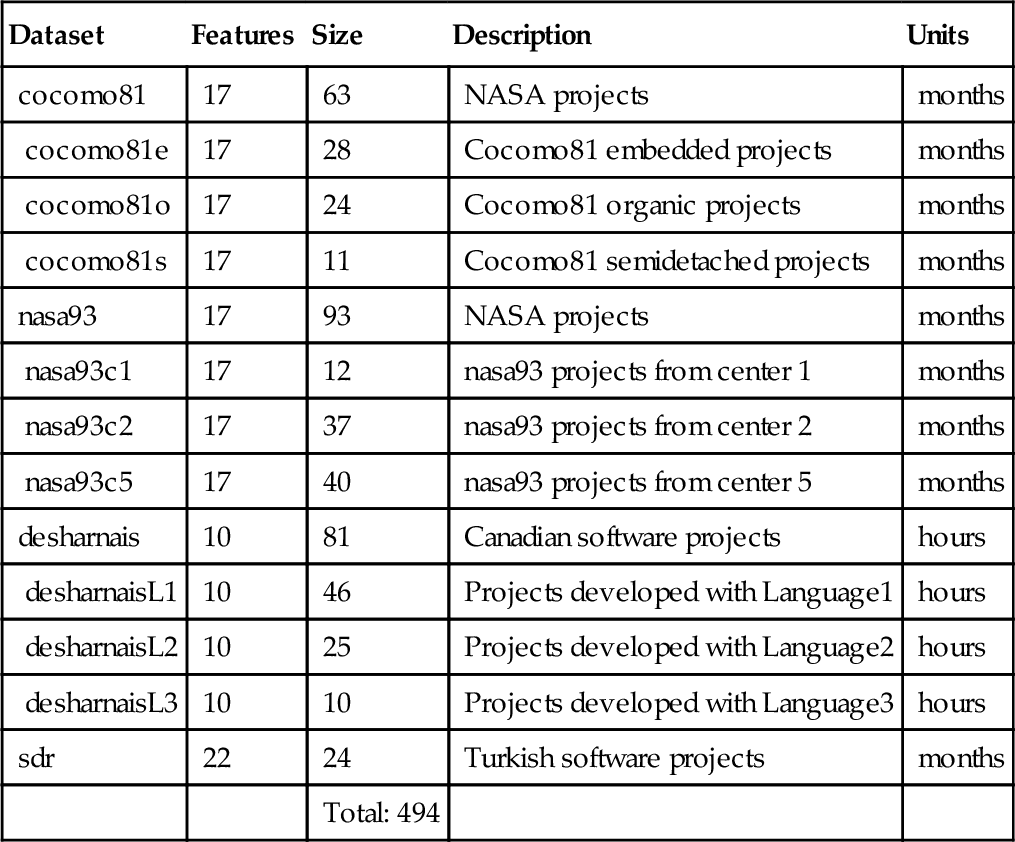
Indentation in column one denotes a data set that is a subset of another data set.
Table 17.2
The Full Data Sets, Their Features, and Collection Methodology
| Methodology | Dataset | Features |
| COCOMO | cocomo81 | RELY, ACAP, SCED |
| cocomo81o | DATA, AEXP, KLOC | |
| cocomo81s | CPLX, PCAP, EFFORT | |
| nasa93 | TIME, VEXP | |
| nasa93c1 | STOR, LEXP | |
| nasa93c2 | VIRT, MODP | |
| nasa93c5 | TURN, TOOL | |
| COCOMOII | sdr | Addition to COCOMO features |
| PREC | ||
| FLEX | ||
| RESL | ||
| TEAM | ||
| PMAT | ||
| FP | desharnais | TeamExp, Effort, Adjustment |
| desharnaisL1 | ManagerExp, Transactions, PointsAjust | |
| desharnaisL2 | YearEnd, Entities, Language | |
| desharnaisL3 | PointsNonAdjust |
The boldface features are identified as size (or size-related) features.
The bold font features in Table 17.2 are identified as size (or size-related) features. These features are removed in reduced data sets. In other words, the full data sets minus the highlighted features gives us the reduced data sets. For convenience, the features that remain after removing the size features are given in Table 17.3. Note that both in Table 17.2 and in Table 17.3, the acronyms of the features are used. These acronyms stand for various software product-related features. For example, COCOMO groups features under six categories:
Table 17.3
The Reduced Data Sets, Their Collection Methodology, and Their Nonsize Features
| Methodology | Dataset | Features |
| COCOMO | cocomo81 | RELY, ACAP, SCED |
| cocomo81o | DATA, AEXP | |
| cocomo81s | CPLX, PCAP, EFFORT | |
| nasa93 | TIME, VEXP | |
| nasa93c1 | STOR, LEXP | |
| nasa93c2 | VIRT, MODP | |
| nasa93c5 | TURN, TOOL | |
| COCOMOII | sdr | Addition to COCOMO features |
| PREC | ||
| FLEX | ||
| RESL | ||
| TEAM | ||
| PMAT | ||
| FP | desharnais | TeamExp, Effort |
| desharnaisL1 | ManagerExp | |
| desharnaisL2 | YearEnd, Language | |
| desharnaisL3 |
Reduced data sets are defined to be the full data sets minus size-related features (boldface features of Table 17.2).
• RELY: Required Software Reliability
• DATA: Database Size
• CPLX: Product Complexity
• RUSE: Required Reusability
• DOCU: Documentation match to life cycle needs
• Platform factors
• TIME: Execution Time Constraint
• STOR: Main Storage Constraint
• PVOL: Platform Volatility
• Personnel factors
• PCAP: Programmer Capability
• PCON: Personnel Continuity
• AEXP: Applications Experience
• PEXP: Platform Experience
• LTEX: Language and Tool Experience
• Project factors
• SITE: Multisite Development
• SCED: Development Schedule
• Input
• Output
• EFFORT: Effort spent for project in terms of man-months
In addition to the original COCOMO method, the improved COCOMOII version defines an additional new category called exponential cost drivers, under which the following features are defined:
• FLEX: Development Flexibility
• RESL: Arch/Risk Resolution
• TEAM: Team Cohesion
• PMAT: Process Maturity
For detailed information and an in depth discussion regarding the above-listed COCOMO and COCOMOII features, refer to Refs. [34, 35]. The FP approach adopts a different strategy than COCOMO. The definitions of the FP data sets (desharnais*) features are as follows:
• TeamExp: Team experience in years
• ManagerExp: Project management experience in years
• YearEnd: The year in which the project ended
• Transactions: The count of basic logical transactions
• Entities: The number of entities in the systems data model
• PointsNonAdjust: Equal to Transactions + Entities
• Adjustment: FP complexity adjustment factor
• PointsAdjust: The adjusted FPs
• Language: Categorical variable for programming language
• Effort: The actual effort measured in person-hours
For more details on these features refer to the work of Desharnais [98] or Li et al. [261]. Note that 4 projects out of 81 in the desharnais data set have missing feature values. Instead of removing these projects from the data set, we employed a missing value handling technique called simple mean imputation [7].
17.2.2 Error measures
Error measures are used to assess the success of a prediction. In this chapter, we stick with the commonly used error measures in SEE.
The absolute residual (AR) is defined as the difference between the predicted and the actual:
where xi and ![]() are the actual and predicted value for test instance i. MAR is the mean of all the AR values.
are the actual and predicted value for test instance i. MAR is the mean of all the AR values.
The magnitude of relative error (MRE) measure is one of the de facto error measures [133, 390]. MRE measures the ratio between the effort estimation error and the actual effort:
A related measure is the magnitude of error relative (MER) to the estimate [133]):
The overall average error of MRE can be derived as the mean or median of MRE, or MMRE and MdMRE, respectively:
A common alternative to MMRE is PRED(25), and it is defined as the percentage of successful predictions falling within 25% of the actual values, and can be expressed as follows, where N is the dataset size:
For example, PRED(25) = 50% implies that half of the estimates are failing within 25% of the actual values [390].
There are many other error measures including mean balanced relative error (MBRE) and the mean inverted balanced relative error (MIBRE) studied by Foss et al. [133]:

We test the numerical comparison of performance measures via a statistical test called the Mann-Whitney rank-sum test (95% confidence). We use Mann-Whitney instead of Student's t-test, as it compares the sums of ranks, unlike Student's t-test, which may introduce spurious findings as a result of outliers in the given data sets.
We use Mann-Whitney to generate win, tie, loss statistics. The procedure used for that purpose is defined in Figure 17.1: First, two distributions i, j (e.g., arrays of MREs or ARs) are compared to see if they are statistically different (Mann-Whitney rank-sum test, 95% confidence); if not, then the related tie values (tiei and tiej) are incremented. If the distributions are different, we update wini, winj and lossi, lossj after error measure comparison.

When comparing the performance of a method (methodi) run on reduced data sets to a method methodj run on full data sets, we will specifically focus on loss values. Note that to make the case for methodi, we do not need to show that its performance is “better” than methodj. We can recommend methodi over methodj as long as its performance is no worse than methodj, i.e., as long as it does not “lose” against methodj.
17.3 Experimental conditions
17.3.1 The algorithms adopted
In this chapter we use two algorithms due their success reported in prior SEE work: a baseline analogy-based estimation method called ABE0 [229] and a decision tree learner called CART [48]. Several papers conclude that CART and nearest-neighbor methods are useful comparison algorithms for SEE. For example, Walkerden and Jeffrey [434] endorse CART as a state-of-the-art SEE method. Dejaeger et al. also claim that, in terms of assessing new SEE methods, methods like CART may prove to be more adequate. The previous work published by the authors is also in the same direction of the conclusions of Walkerden, Jeffrey, Dejaeger et al. Our 2011 study reports an extensive comparison of 90 SEE methods (generated using all combinations of 10 preprocessors and 9 learners) [223]. In this study the most successful SEE methods turn out to be ABE0 with 1-nearest neighbor (which will be referred to as 1NN from now on) and CART.
ABE methods generate an estimate for a future project by retrieving similar instances among past projects. Then the effort values of the retrieved past projects are adapted into an estimate. There are various design options associated with ABE methods, yet a basic ABE method can be defined as follows:
• Input a database of past projects.
• For each test instance, retrieve k similar projects (analogies) according to a similarity function.
• Adapt the effort values of the k nearest analogies to come up with the effort estimate.
ABE0 uses the Euclidean distance as a similarity measure, whose formula is given in Equation (17.9), where wi corresponds to feature weights applied on independent features fAi and fBi of instances A and B, respectively. t is the total number of independent features. ABE0 framework equally favors all instances, i.e., wi = 1. For adaptation, ABE0 takes the median of retrieved k projects. The ABE0 adopted in this research uses a 1-nearest neighbor (i.e., k = 1); hence, the name 1NN.
Iterative dichotomizers like CART find the feature that most divides the data such that the variance of each division is minimized [48]. The algorithm then recurses into each division. Once the tree is generated, the cost data of the instances in the leaf nodes are averaged to generate an estimate for the test case. For more details on CART, refer to Breiman et al. [48].
17.3.2 Proposed method: POP1
The 1NN variant proposed in this chapter utilizes the popularity of the instances in a training set. We define the “popularity” of an instance as the number of times it happens to be the nearest neighbor of other instances. The proposed method is called POP1 (short for popularity-based-1NN). The basic steps of POP1 can be defined as follows:
Step 1: Calculate distances between every instance tuple in the training set.
Step 2: Convert distances of step 1 into ordering of neighbors.
Step 3: Mark closest neighbors and calculate popularity.
Step 4: Order training instances in decreasing popularity.
Step 5: Decide which instances to select.
Step 6: Return estimates for the test instances.
The following paragraphs describe the details of each step:
Step 1: Calculate distances between every instance tuple in the training set. This step uses the Euclidean distance function (as in 1NN) to calculate the distances between every pair of instances within the training set. The distance calculation is kept in a matrix called D, where ith row keeps the distance of the ith instance to other instances. Note that this calculation requires only the independent features. Furthermore, because POP1 runs on reduced data sets, size features are not used in this step.
Step 2: Convert distances of Step 1 into ordering of neighbors. This step requires us to merely replace the distance values with their corresponding rank from the closest to the farthest. We work one row at a time on matrix D: Start from row #1, rank distance values in ascending order, then replace distance values with their corresponding ranks, which gives us the matrix D′. The ith row of D′ keeps the ranks of the neighbors of the ith instance.
Step 3: Mark closest neighbors and calculate popularity. Because POP1 uses only the closest neighbors, we leave the cells of D′ that contain 1 (i.e., that contain a closest neighbor) untouched and replace the contents of all the other cells with zeros. The remaining matrix D″ marks only the instances that appeared as the closest neighbor to another instance.
Step 4: Order training instances in decreasing popularity. This step starts summing up the “columns” of D″. The sum of, say, ith column shows how many times the ith instance was marked as the closest neighbor to another instance. The sum of the ith column equals the popularity of the ith instance. Finally, in this step we rank the instances in decreasing popularity, i.e., the most popular instance is ranked #1, the second is ranked #2, and so on.
Step 5: Decide which instances to select. This step tries to find how many of the most popular instances will be selected. For that purpose we perform a 10-way cross-validation on the train set. For each cross-validation (i.e., 10 times), we do the following:
• Perform steps 1-4 for the popularity order.
• Build a set S, into which instances are added one at a time from the most popular to the least popular.
• After each addition to S make predictions for the hold-out set, i.e., find the closest neighbor from S of each instance in the hold-out set and use the effort value of that closest instance as the estimate.
• Calculate the error measure of the hold-out set for each size of S. As the size of S increases (i.e., as we place more and more popular instances into S) the error measure is expected to decrease.
• Traverse the error measures of S with only one instance of S with t instances (where t is the size of the training set minus the hold-out set). Mark the size of S (represented by s′) when the error measure has not decreased more than Δ for n-many consecutive times.
Note that because we use a 10-way cross-validation, at the end of the above steps we will have 10 s′ values (1 s′ value from each cross-validation). We take the median of these values as the final s′ value. This means that POP1 only selects the most popular s′-many instances from the training set. For convenience, we refer to the new training set of selected s′-many instances as Train′.
Step 6: Return estimates for the test instances. This step is fairly straightforward. The estimate for a test instance is the effort value of its nearest neighbor in Train′ (Figure 17.2).

For the error measure in Step 5, we used MRE, which is only one of the many possible error measures. As shown in Section 17.4, even though we guide the search using only MRE, the resulting estimations score very well across a wide range of error measures. In the following experiments, we used n = 3 and Δ < 0.1. The selection of (n, Δ) values is based on our engineering judgment. The sensitivity analysis of (n, Δ) values can be a promising future work.
17.3.3 Experiments
So as to observe the performance of the proposed POP1 method in terms of compensating for the lack of size attributes, we designed a two-stage experimentation: (1) 1NN and CART performances on reduced data sets compared to their performance on full data sets; (2) POP1 performance on reduced data sets compared to 1NN and CART performance on full data sets.
In the first stage we question whether standard SEE methods can compensate for mere removal of the size features. For that purpose, we run 1NN as well as CART on reduced and full data sets separately through 10-way cross-validation. Then each method's results on reduced data sets are compared to its results on full data sets. The outcome of this stage tells us whether there is a need for POP1-like methods or not. If the performance of CART and 1NN on reduced data sets are statistically the same as their performances on the full data sets, then this would mean that standard successful estimation methods are able to compensate for the lack of size features. However, as we see in Section 17.4, that is not the case. The removal of size features has a negative effect on 1NN and CART.
The second stage tries to answer whether simple SEE methods like 1NN can be augmented with a preprocessing step, so that the removal of size features can be tolerated. For that purpose we run POP1 on the reduced data sets and compare its performance to 1NN and CART (run on full data sets) through 10-way cross-validation. The performance is measured in 7 error measures.
17.4 Results
17.4.1 Results without instance selection
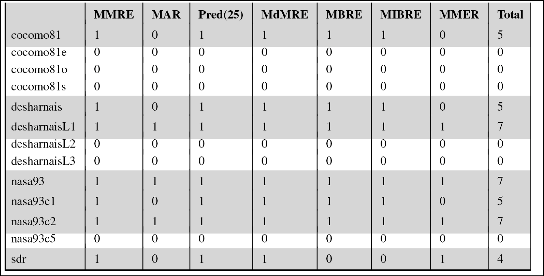
Table 17.4 shows the CART results for the first stage of our experimentation, i.e., whether or not standard estimation methods, in that case CART, can compensate for the lack of size. In Table 17.4 we compare CART run on reduced data sets to CART run on full data sets and report the loss values. The loss value in each cell is associated with an error measure and a data set. Each loss value shows whether CART on reduced data lost against CART on full data. Note that it is acceptable for CART-on-reduced-data, as long as it does not lose against CART-on-full-data, Because we want the former to perform just as well as (not necessarily better than) the latter. The last column of Table 17.4 is the sum of the loss values over 7 error measures. The rows in which CART on reduced data loses for most of the error measures (4 or more out of 7 error measures) are highlighted. See in Table 17.4 that 7 out of 13 data sets are highlighted; i.e., more than half the time CART cannot compensate the lack of size features.
Table 17.4
The Loss Values of CART Run on Reduced Data Set vs. CART Run on Full Data Set, Measured Per Error Measure
 |
From Ref. [230].
The last column shows the loss values in the total of 7 error measures. The data sets where CART is running on reduced data sets lose more than half the time (i.e., 4 or more out of 7 error measures) against CART running on full data sets are highlighted.
Although Table 17.4 is good to see the detailed loss information, the fundamental information we are after is summarized in the last column: total loss number. Repeating Table 17.4 for all the methods in both stages of the experimentation is cumbersome and would redundantly take too much space in this chapter. Hence, from now on we will use summary tables as given in Table 17.5, which shows only the total number of losses. Note that the “CART” column of Table 17.5 is just the last column of Table 17.4. Aside from the CART results, Table 17.5 also shows the loss results for 1NN run on reduced data vs. 1NN run on full data. The highlighted cells of the “1NN” column show the cases where 1NN lost most of the time, i.e., 4 or more out of 7 error measures. Similar to the results of CART, 1NN-on-reduced-data loses against 1NN-on-full-data for 7 out of 13 data sets. In other words, for more than half the data sets mere use of 1NN cannot compensate for the lack of size features.
Table 17.5
The Loss Values of Estimation Methods Run on Reduced Data Sets vs. Run on Full Data Sets
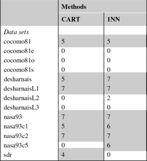 |

The cases where reduced data set results lose more than half the time (i.e., 4 or more out of 7 error measures) are highlighted.
The summary of the first stage of experimentation is that standard SEE methods are unable to compensate for the size features for most of the data sets experimented in this chapter. In the next section we show the interesting result that it is possible to augment a very simple ABE method like 1NN so that it can compensate for size features in a great majority of the data sets.
17.4.2 Results with instance selection
The comparison of POP1 (which runs on reduced data sets) to 1NN and CART (which run on full data sets) is given in Table 17.6. Table 17.6 shows the total loss values of POP1 over 7 error measures, so the highest number of times POP1 can lose against 1NN or CART is 7. The cases where POP1 loses more than half the time (i.e., 4 or more out of 7 error measures) are highlighted.
Table 17.6
The Loss Values of POP1 vs. 1NN and CART Over 7 Error Measures
 |

The data sets where POP1 (running on reduced data sets) lose more than half the time (i.e., 4 or more out of 7 error measures) against 1NN or CART (running on full data sets) are highlighted.
The comparison of POP1 against 1NN shows whether the proposed POP1 method helps standard ABE methods to compensate for the lack of size features. Note that in the second column of Table 17.6 there are only two highlighted cells. For 11 out of 13 data sets, the performance of POP1 is statistically the same as that of 1NN. The only two data sets, where POP1 cannot compensate for size are cocomo81e and desharnais.
The fact that POP1 compensates for size in cocomo81e's superset (cocomo81) and in desharnis' subsets (desharnaisL1, desharnaisL2, and desharnaisL3) but not in these two data sets may at first seem puzzling, because the expectation is that subsets share similar properties as their supersets. However, a recent work by Posnett et al. has shown that this is not necessarily the case [361]. The focus of Posnet et al.'s work is the “ecological inference”; i.e., the delta between the conclusions drawn from subsets vs. the conclusions from the supersets. They document the interesting finding that conclusions from the subsets may be significantly different than the conclusions drawn from the supersets. Our results support their claim that supersets and subsets may have different characteristics.
The last column of Table 17.6 shows the number of times POP1 lost against CART. Again, the cases where POP1 loses for more than 4 error measures are highlighted. The purpose of POP1's comparison to CART is to evaluate a simple ABE method like POP1 against a state-of-the-art learner like CART. As can be seen in Table 17.6, there are four highlighted cells under the last column, i.e., for 13 − 4 = 9 data sets, the performance of POP1 is statistically identical to that of CART. This is an important result for two reasons: (1) a simple ABE method like POP1 can attain performance values as good as CART for most of the data sets and (2) the performance of POP1 comes from data sets without any size features.
17.5 Summary
The implication of the POP1 algorithm presented in this chapter should not be taken as a proposition to deprecate the use of size attributes. There are still a many parametric methods that are in practical use such as COCOMO and FP. On the other hand, in the case of SEE, it is possible to tolerate the lack of size features, given that an instance selection mechanism selects only the relevant instances. We evaluate 1NN and CART, which are reported as the best methods out of 90 methods in a prior SEE study [223]. Our results show that the performance of 1NN and CART on reduced data sets is worse than their performance on full data sets. Hence, mere use of these methods without size features is not recommended.
Then we augmented 1NN with a popularity-based preprocessor to come up with POP1. We run POP1 on reduced data sets and compare its performance to 1NN and CART, which are both run on full data sets. The results of this comparison show that for most of the cases (11 out of 13 data sets), POP1 running on reduced data sets attains the same performance as its counterpart 1NN running on full data sets.
Size features are essential for standard learners such as 1NN and CART. SEE practitioners with enough resources to collect accurate size features should do so. On the other hand, when standard learners (in this research it is 1NN) are augmented with preprocessing options (in this research it is a popularity-based preprocessor), it is possible to remove the necessity of size features. Hence, SEE practitioners without sufficient resources to measure accurate size features should consider alternatives like POP1. Note that the proposed method was built on a successful learner on SEE data sets. Hence, if ABE methods are poor performers for the data sets of your domain, it may be a disappointing trial to stick with 1NN on such a domain. The recommendation for such a case would be to
• Identify high-performing learners on the data sets of your domain.
• Identify biases of these learners and how they can be utilized in the context of instance selection.
• Augment and utilize the identified biases to propose an ordering of the training instances (e.g., the similarity idea and the decision trees we discussed in the introduction).