5.1 Controlling Data Collection

All inductive agents (be they human or artificial) can make inductive errors, so we must employ some methods to minimize the frequency of those errors. The standard approach to this problem is to use some initial requirements at the gathering stage where the goals of the learning are defined in a careful and reflective way, as discussed in:

• Basili's Goal-Question-Metric [283] approach;

• and Easterbrook et al.'s notes on empirical SE [110].

The intent of this standard approach is to prevent spurious conclusions by (a) carefully controlling data collection and by (b) focusing the investigation on a very small space of hypotheses. Where possible, we strongly recommend this controlled approach to data collection. But what to do if such control is not possible?

5.2 Problems With Controlled Data Collection

In practice, full control over data collection is not always possible. Collecting data comes at a cost, for example:

• Data collection should not stress the available hardware resources. For example, the transmission of that data should not crash the network. Further, the storage of that data should not exceed the free space on the hard drives.

• If humans are involved in that data collection, the effort associated with that collection must not detract from normal operations.

For these reasons, it is infeasible to collect all possible data. Worse, in our experience, it may not be possible to control data collection even for the limited amounts of information you can receive. For example, when one of us (Menzies) tried collecting data from inside NASA, he found many roadblocks to data collection. NASA makes extensive use of large teams of contractors. Data collection across those teams must navigate many layers of management from subcontractors and sub-subcontractors. This means that communication to data owners had to be mediated by up to a dozen account managers, all of whom may have many higher priority tasks to perform. Hence, very little data was ever transferred to Menzies. Further, when data was transferred, there were very few knowledgeable humans available who could discuss the content of that data.

Even when restricted to within one organization, data collection can also be complicated and exorbitantly expensive. Jairus Hihn reports the $1.5 million NASA spent in the period 1987-1990 to understand the historical records of all their software. In that study, five NASA analysts (including Hihn) worked half-time to fully document 200 records describing NASA's software development experience. NASA analysts traveled around the country to interview contractors and collect meta-knowledge about a spreadsheet of 200 rows and less than 30 columns. At the end of this process, the analysts wrote four fat volumes (300+ pages each) reporting their conclusions. Hihn reported that this exercise has never been repeated because it was so expensive [173].

Consequently, in many cases, a data scientist must

Hence, the task of the data scientist is to make the most of the data at hand, and not wait for some promised future data set that might never arrive.

5.3 Rinse (and Prune) Before Use

We may not have control over how data is collected, so it is wise to cleanse the data prior to learning. Happily, a standard result is that given a table of data, 80-90% of the rows and all but the square root of the number of columns can be deleted before comprising the performance of the learned model [71, 155, 221, 234]. That is, even in dirty data sets it is possible to isolate and use “clean” sections. In fact, as we show below, removing rows and columns can actually be beneficial to the purposes of data mining.

5.3.2 Column Pruning

The case for pruning columns is slightly more complex.

Undersampling. The number of possible influences on a project is quite large and, usually, historical data sets on projects for a particular company are quite small. Hence, a variable that is theoretically useful may be practically useless. For example, Figure 5.1 shows how, at one NASA site, nearly all the projects were rated as having a high complexity (see Figure 5.1).
Therefore, this data set would not support conclusions about the interaction of, say, extra highly complex projects with other variables. A learner would be wise to subtract this variable (and a cost modeling analyst would be wise to suggest to their NASA clients that they refine the local definition of “complexity”).

Reducing Variance. Miller offers an extensive survey of column pruning for linear models and regression [316]. That survey includes a very strong argument for column pruning: the variance of a linear model learned by minimizing least squares error decreases as the number of columns in is decreased. That is, the fewer the columns, the more restrained are the model predictions.

Irrelevancy. Sometimes, modelers are incorrect in their beliefs about what variables effect some outcome. In this case, they might add irrelevant variables to a database. Without column pruning, a model learned from that database might contain these irrelevant variables. Anyone trying to use that model in the future would then be forced into excessive data collection.

Noise. Learning a model is easier when the learner does not have to struggle with fitting the model to confusing noisy data (i.e., when the data contains spurious signals not associated with variations to projects). Noise can come from many sources such as clerical errors or missing data. For example, organizations that only build word processors may have little data on software projects with high reliability requirements.

Correlated Variables. If multiple variables are tightly correlated, then using all of them will diminish the likelihood that either variable attains significance. A repeated result in data mining is that pruning away some of the correlated variables increases the effectiveness of the learned model (the reasons for this are subtle and vary according to which particular learner is being used [155]).

5.4 On the Value of Pruning

This section offers a case study about the benefits of row and column pruning in software effort estimation. The interesting thing about this example is that pruning dramatically improved the predictions from the model, especially for the smaller data sets. That is, for these data sets, the paradoxical result is this:

• The less data you have, the more you need to throw away.

This study [75] uses data sets in Boehm's COCOMO format [34, 42]. That format contains 15-22 features describing a software project in terms of its personnel, platform, product and use in a project. In this study, the projects were of difference sizes:

• For example, the largest data set had 160 projects;

• And the smallest had around a dozen.

Feature reduction was performed on all these data sets using a column pruner called WRAPPER. This WRAPPER system calls for some “wrapped” learner (in this case, linear regression) on some subset of the variables. If the results look promising, WRAPPER then grows that subset till the performance stops improving. Initially, WRAPPER starts with subsets of size one (i.e., it tries every feature just on its on).

Figure 5.2 shows how many columns were thrown away from each data set (all the data sets are sorted on the x-axis sorted left to right, largest to smallest). In that figure, the solid and dotted lines of show the number of columns in our data sets before and after pruning:

• In the original data sets, there were 22 attributes. For the largest data set shown on the left-hand side of Figure 5.2, WRAPPER did nothing at all (observe how the red and green lines fall to the same left-hand side point; i.e., WRAPPER kept all 22 columns).

• However, as we sweep from left to right, largest data set to smallest, we see that WRAPPER threw away more columns from the smaller data sets (with one exception—see the p02 data set, second from the right).

This is a strange result, to say the least; the smaller data sets were pruned the most. This result raises the question: Is the pruning process faulty?

To test that, we computed the “PRED(30)” results using all columns and just the reduced set of columns. This PRED(30) error message is defined as follows:

• PRED(30) = the percent of estimates that were within 30% of actual.

• For example, a PRED(30) = 50% means that half the estimates are within 30% of the actual.

The PRED(30) results associated with the pruned data sets are shown in Figure 5.3:

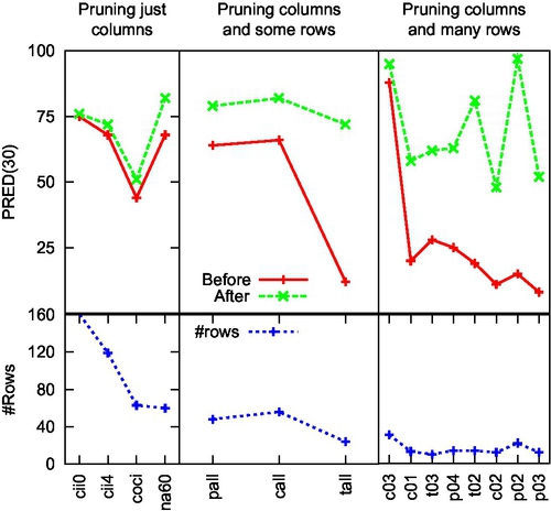
• The Solid lines on Figure 5.3 show the mean PRED(30) seen in 30 trials using all the columns. These are the baseline results for learning cost models before applying any pruning method.

• The dotted lines show the mean PRED(30) seen after automatic column pruning.

• The difference between the solid and the dotted lines is the improvement produced by pruning.

The key observation from this result is that if you start with less data, then the more columns you throw away, the better the final predictions. Why is this so? The answer comes from the mathematics of curve fitting:

• A model is a fit of some shape to a set of data points.

• Each feature is a degree of freedom along which the shape can move.

• If there are more degrees of freedom than original data points, then the shape can move in many directions. This means that there are multiple shapes that could be fitted to the small number of points.

That is, to clarify a model learned from a limited data source, prune that data source.

5.5 Summary

Certainly, it is useful to manually browse data in order to familiarize yourself with the domain and conduct “sanity checks” within the data. But data may contain “islands” of interesting signals surrounded by an ocean of confusion. Automatic tools can extract those interesting humans, thus topping humans from getting confused by the data.

This notion of pruning irrelevancies is a core concept of data mining, particularly for human-in-the-loop processes. Later in this book, we offer more details on how to conduct such data pruning (see Chapters 10 and 15).