
The Importance of Goals in Model-Based Reasoning
Abstract
In this part of the book Data Science for Software Engineering: Sharing Data and Models, explores ensemble learners and multi-objective optimizers as applied to software engineering. Novel incremental ensemble learners are explained along with one of the largest ensemble learning (in effort estimation) experiments yet attempted. It turns out that the specific goals of the learning has an effect on what is learned and, for this reason, this part also explores multi-goal reasoning. We show that multi-goal optimizers can significantly improve effort estimation results.
In summary, this chapter proposes the following data analysis pattern:
| Name: | SEESAW |
| Also known as: | Optimizer, constraint solver. |
| Intent: | Reasoning about a software process model. |
| Motivation: | The managers of software projects can make a very large number of decisions about those projects. |
| Solution: | Exploring all those options is a task better done by automatic methods, if only to whittle down thousands of options to just a few. |
| Constraints: | Different kinds of projects have different definitions of what is “best.” |
| Implementation: | Rather than hardwire a rigid definition of “best” into our search algorithms, make “best” a domain-specific predicate that can be altered for different contexts. |
| Applicability: | SEESAW can produce recommendations about how to change a project that are tuned to the particulars of the goals of different projects. Those recommendations are radically different for different goals. Hence, rather than offer some trite “one-size-fits-all” solution for all projects, it is better to reason about the specifics of the local project. |
| Related to: | SEESAW uses an aggregation function to combine N goals into a single optimization goal. The optimizers of Chapter 24 can generate solutions across the frontier of best solutions over the space of all aggregation functions. |
This chapter is an extension of a paper “Understanding the Value of Software Engineering Technologies” by Phillip Green, Tim Menzies, Steven Williams, and Oussama El-Rawas presented at the 2009 IEEE/ACM International Conference on Automated Software Engineering. This chapter adds extensive notes on the business implications and context of this work.
23.1 Introduction
This book is about sharing data and sharing models. A premise of share is that sharing is useful; i.e., if I give something to you, then you can look at it and say “yes, I understand.” The message of this chapter is that unless we share the same values, then it is hard for you to see the value in what is shared. So this chapter is all about values and how different values can contort what is considered or useful.
This chapter presents a case study where a software process is explored using different values. Prior to work, we had a preexperimental intuition that concepts of value might change the organization of a project. However, we suspected that some things would remain constant, such as
• Condoning the use of execution testing tools.
• Encouraging increasing software process maturity.
This turned out not to be the case. In the case study for this chapter, for the value functions explored here, if one function approves of X then the other usually approves of not X.
This result, that value can change everything, should motivate the reader to spend more time on understanding and recording their own values, as well as the values of anyone with which they want to share data or models. This is important as sharing is unlikely between teams that have very different value systems.
23.2 Value-based modeling
23.2.1 Biases and models
To understand the flow of this chapter, the reader might want to first reread Chapter 3. That chapter remarked that any inductive process is fundamentally biased. That is, human reasoning and data mining algorithms search for models in their own particular biased way. This is unavoidable as the space of models that can be generated from any data set is very large. If we understand and apply user goals, then we can quickly focus a data mining project on the small set of most crucial issues. Hence, it is vital to talk to users in order to lever age their biases to better guide the data mining. The lesson of this chapter is that bias is a first-class modeling construct. It is important to search out, record, and implement biases because, as shown below, different biases lead to radically different results.
23.2.2 The problem with exploring values
In software engineering, biases are expressed as the values business users espouse for a system. Barry Boehm [41] advocated assessing software development technologies by the value they give to particular stakeholders. Note that this is very different from the standard practice (which assesses technologies via their functionality).
In his description of value-based SE, Boehm favors continuous optimization methods to conduct cost/benefit trade-off studies. Translated into the terminology of this book, he is advocating data mining methods that are tuned to different value propositions.
A problem with this kind of trade-off is that it must explore some underlying space of options. In a conventional approach, some business process model could be developed, then exercised many times. Such a data farming approach
1. Plants a seed. Build a model from domain information. All uncertainties or missing parts of the domain information are modeled as a space of possibilities.
2. Grows the data. Execute the model and, when the model moves into the space of possibilities, output is created by selecting at random from the possibilities.
3. Harvests. Summarize the grown data via data mining.
4. Optionally, use the harvested summaries to improve the model; then, go to 1.
There are two problems with the above approach:
• Tuning instability (that complicates the above step 2);
• Value variability (that complicates the above step 3).
Tuning instability refers to the problem of tuning a model to some local domain. Ideally, there is enough local data to clearly define what outputs are expected from a model. In practice, this may not be the case so the second step of data farming, grow the data, results in very large variances in model performance.
Value variability is the point of this chapter. After doing everything we can to tame tuning instability, we still need to search the resulting space of options in order to make a recommendation that is useful for the user. If, during the third step (harvest), we change the value proposition used to guide that search then we get startlingly different recommendations.
The next two sections offer more details on tuning instability and value variability. While these two terms have many differences, they relate to a similar concept:
• Tuning instability refers to uncertainties inside a model;
• Value variability refers to uncertainty on how to assess the outputs of a model.
23.2.2.1 Tuning instability
In theory, software process models can be used to model the trade-offs associated with different technologies. However, such models can suffer from tuning instability. Large instabilities make it hard to recognize important influences on a project. For example, consider the following simplified COCOMO [42] model,
While simplified, the equation presents the core assumption of COCOMO; i.e., that software development effort is exponential on the size of the program. In this equation, (a, b) control the linear and exponential effects (respectively) on model estimates; while pmat (process maturity) and acap (analyst capability) are project choices adjusted by managers. Equation (23.1) contains two features (acap, pmat) and a full COCOMO-II model contains 22 [42].
Baker [19] reports a study that learned values of (a, b) for a full COCOMO model using Boehm's local calibration method [34] from 30 randomly selected samples of 90% of the available project data. The ranges varied widely:
Such large variations make it possible to misunderstand the effects of project options. Suppose some proposed technology doubles productivity, but a moves from 9 to 4.5. The improvement resulting from that change would be obscured by the tuning variance.
(For more on the issue of tuning instability in effort estimation, the reader could refer back to Figure 1.2.)
23.2.2.2 Value variability
Another source of variability in a model are the goals (a.k.a. values) used to generate that model. There are a surprisingly large number of ways to assess the outputs of models of software systems. For example, consider something as seemingly simple as a defect predictor. Such detectors read code and point to regions with larger odds of having bugs. What could be simpler than that?
As it turns out, defect predictors can be assessed on many criteria such as those listed in Figure 23.1. In that figure, support comments on how much training data was used to build this detector. Also, effort looks at how many lines of code are selected by the detector. Finally, reward comments on the ease of finding bugs. If reward is high, then an analyst can find many bugs after reading a small part of the code.
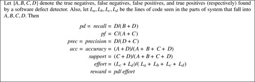
Figure 23.2 lists other performance measures that we have seen at client sites or in the literature. There are two important features of this figure:

2. This list keeps growing.
As to this second point, often when we work with new clients, they surprise us with yet another domain-specific criteria that is important for the business. That is, neither Figure 23.1 nor Figure 23.2 is a complete list of all possible assessment criteria.
Our reading of the software engineering literature is that most papers only explore a small subset of Figure 23.1 or Figure 23.2. We think this is a mistake, and researchers should do more to create a more general framework where they explore a wide and changing set of evaluation criteria. The next section describes one such framework.
23.2.2.3 Exploring instability and variability
To address the above problems, we adopt two strategies:
• To address value variability we
• Use tools that allow for the customization of the value proposition used to guide the search.
• Then run the models using different value propositions.
• To address tuning instability we
• Determine the space of known tunings for a model.
• Allow models to range over that space.
• Extensively simulate the models.
• Look for stable conclusions over the entire space of tunings.
The rest of this chapter offers an example of this kind of analysis.
23.3 Setting up
To apply the above exploration rules, we first need to
• Represent multiple value propositions.
• Represent the space of options.
This setting up section discusses one way to implement those representations.
23.3.1 Representing value propositions
A value function should model the goals of the business users who are making project decisions about some software development. We will explore two:
• BFC = Better, faster, cheaper.
• XPOS = Risk exposure.
Value proposition #1- Better, faster, cheaper (BFC). Ideally, software is built with fewer defects D, using less effort E, and in shorter time T. A value function for this goal can be modeled as the Euclidean distance to minimum effort, time, defects:

In the above, value is highest when defects and effort and development time are lowest. Also, 0 ≤ (b, f, c) ≤ 1 represents the business importance of (better, faster, cheaper). For this study, we use b = f = c = 1. In other work, we have explored the effects of using other b, f, and c values [304].
In Equation (23.3), ![]() ,
, ![]() , and
, and ![]() are the time, effort, and defect scores normalized zero to one. Equation (23.3) models the business intuition that defects in high-reliability systems are exponentially more troublesome than in low-reliability systems:
are the time, effort, and defect scores normalized zero to one. Equation (23.3) models the business intuition that defects in high-reliability systems are exponentially more troublesome than in low-reliability systems:
• In the COCOMO model, variables have the range 1 ≤ x ≤ 6 and at x = 3, the variable's influence on the output is nominal; in other words, its impact on effort is to multiply it by one (which is to say, it leaves it unchanged).
• In the COCOMO model, if reliability moves from very low to very high (1 to 6), the term 1.8rely–3 models a function that (a) is ten times larger for very high than very low reliability systems; and (b) passes through 1 at rely = 3 (so systems with nominal reliability do not change the importance of defects).
Value proposition #2- Risk exposure (XPOS). The BFC value function is somewhat idealistic in that it seeks to remove all defects by spending less money on faster developments. An alternate value function comes from Huang and Boehm [183]. This alternate value function, which we call XPOS, models the situation where a software company must rush a product to market, without compromising too much on software quality. Based on Huang's PhD dissertation [182], we operationalize XPOS as follows.
Huang defines business risk exposure (RE) as a combination of software quality investment risk exposure (REq) and market share erosion risk exposure (REm). We invert that expression to yield valueXPOS (so an exposed project has low value):
REq values high-quality software and therefore prioritizes quality over time. REq is composed of two primary components: probability of loss due to unacceptable quality Pq(L) and size of loss due to unacceptable quality Sq(L). Pq(L) is calculated based on defects. Sq(L) is calculated based on complexity (the COCOMO cplx feature), reliability (rely), and a cost function. Sc is a value from a Pareto-valued table based on rely. We choose the project months estimate as the basis of this cost function.

In Equation (23.8), defectsvl is the lower bound on defects for that project.
In Equation (23.9), the  term is similar to the
 ![]() coefficient inside Equation (23.3): if complexity changes below or above 3, then it reduces or adds (respectively) to the unacceptable quality risk. However, at cplx = 3, the multiplier is one (i.e., no effect).
coefficient inside Equation (23.3): if complexity changes below or above 3, then it reduces or adds (respectively) to the unacceptable quality risk. However, at cplx = 3, the multiplier is one (i.e., no effect).
REm values a fast time-to-market and therefore prioritizes time over quality. REm is calculated from PM and reliability (rely). Mc is a value from a exponential-valued table based on rely.
23.3.1.1 Representing the space of options
How do we allow models to range over the space of known tunings? To answer that question, we need to understand something about models. The predictions of a model about a software engineering project are altered by project variables P and tuning variables T:
For example:
• In Equation (23.1), the tuning options T are the range of (a, b) and the project options P are the range of pmat (process maturity) and acap (analyst capability).
• Given what we know about the COCOMO model, we can say that the ranges of the project variables are P = 1 ≤ (pmat, acap) ≤ 5.
• Given the cone of uncertainty associated with a particular project p, we can identify the subset of the project options p ⊆ P relevant to a particular project. For example, a project manager may be unsure of the exact skill level of team members. However, if she were to assert “my analysts are better than most,” then p would include {acap = 4, acap = 5}.
Next, we make the following assumption:
The dominant influences on the prediction are the project options p (and not the tuning options T).
Under this assumption, the predictions can be controlled by
• Constraining p (using some AI tool);
• While leaving T unconstrained (and sampling t ∈ T using Monte Carlo methods).
Specifically, we seek a treatment rx ⊆ p that maximizes the value of a model's predictions where value is a domain-specific function that scores model outputs according to user goals:

23.4 Details
The last section offered, in broad strokes, an outline of how to handle tuning instability and value variability. To operationalize that high-level picture, we must now move into the inner details of a specific model.
The rest of this chapter is based on an example taken from the USC COCOMO suite of project management tools [36]:
• The COCOMO model offers effort and time predictions.
• The COQUALMO offers defect predictions.
Using the models, we can represent the project options P and tuning options T of Equation (23.11) as follows.
23.4.1 Project options: P
COCOMO and COQUALMO's features are shown in Figure 23.3 and Figure 23.4. The features have a range taken from {very low, low, nominal, high, very high, extremely high} or
These features include manual methods for defect removal. High values for peer reviews (or pr, see Figure 23.4) denote formal peer group review activities (participants have well-defined and separate roles, the reviews are guided by extensive review checklists/root cause analysis, and reviews are a continuous process guided by statistical control theory [397]).


COQUALMO also models automatic methods for defect removal. Chulani [99] defines the top half of automated analysis as
4 (high): intermediate-level module and intermodule code syntax and semantic analysis. Simple requirements/design view consistency checking.
5 (very high): More elaborate requirements/design view consistency checking. Basic distributed processing and temporal analysis, model checking, symbolic execution.
6 (extremely high): Formalized1 specification and verification. Temporal analysis, model checking, symbolic execution.
The top half of execution-based testing and tools is
4 (high): Well-defined test sequence tailored to organization (acceptance / alpha / beta / flight / etc.) test. Basic test coverage tools, test support system.
5 (very high): More advanced tools, test data preparation, basic test oracle support, distributed monitoring and analysis, assertion checking. Metrics-based test process management.
6 (extremely high): Highly advanced tools: oracles, distributed monitoring and analysis, assertion checking. Integration of automated analysis and test tools. Model-based test process management.
In the sequel, the following observation will become important: Figure 23.3 is much longer than Figure 23.4. This reflects a modeling intuition of COCOMO/COQUALMO: it is better to prevent the introduction of defects (using changes to Figure 23.3) than to try and find them once they have been introduced (using Figure 23.4).
23.4.2 Tuning options: T
For COCOMO effort multipliers (the features that that affect effort/cost in a linear manner), the off-nominal ranges {vl=1, l=2, h=4, vh=5, xh=6} change the prediction by some ratio. The nominal range {n=3}, however, corresponds to an effort multiplier of 1, causing no change to the prediction. Hence, these ranges can be modeled as straight lines y = mx + b passing through the point (x, y)=(3, 1). Such a line has a y-intercept of b = 1 − 3m. Substituting this value of b into y = mx + b yields:
where mα is the effect of α on effort/cost.
We can also derive a general equation for the features that influence cost/effort in an exponential manner. These features do not “hinge” around (3,1) but take the following form:
where mβ is the effect of factor i on effort/cost.
COQUALMO contains equations of the same syntactic form as Equation (23.13) and Equation (23.14), but with different coefficients. Using experience for 161 projects [42], we can find the maximum and minimum values ever assigned to m for COQUALMO and COCOMO. Hence, to explore tuning variance (the t ∈ T term in Equation (23.12)), all we need to do is select m values at random from the min/max m values ever seen.
23.5 An experiment
This section describes an experiment where the value propositions of Section 23.3.1 are applied to the model described in Section 23.3.1.1 and Section 23.6.
23.5.1 Case studies: p ⊆ P
We use p to denote the subset of the project options pi ⊆ P relevant to particular projects. The four particular projects p1, p2, p3, p4 used as the case studies of this chapter are shown in Figure 23.5:

• OSP is the GNC (guidance, navigation, and control) component of NASA's Orbital Space Plane.
• OSP2 is a later version of OSP.
• Flight and ground systems reflect typical ranges seen at NASA's Jet Propulsion Laboratory.
Some of the features in Figure 23.5 are known precisely (see all the features with single fixed settings). But many of the features in Figure 23.5 do not have precise settings (see all the features that range from some low to high value). Sometimes the ranges are very narrow (e.g., the process maturity of JPL ground software is between 2 and 3), and sometimes the ranges are very broad.
Figure 23.5 does not mention all the features listed in Figure 23.3 inputs. For example, our defect predictor has inputs for use of automated analysis, peer reviews, and execution-based testing tools. For all inputs not mentioned in Figure 23.5, ranges are picked at random from (usually) {1, 2, 3, 4, 5}.
23.5.1.1 Searching for rx
Our search runs two phases: a forward select and a back select phase. The forward select grows rx, starting with the empty set. At each round i in the forward select one or more ranges (e.g., acap = 3) are added to rx. The resulting rx set found at round i is denoted rix.
The forward select ends when the search engine cannot find more ranges to usefully add to rix. Before termination, we say that the open features at round i are the features in Figure 23.3 and Figure 23.4 not mentioned by any range in rix. The value of rix is assessed by running the model N times with
2. Any t ∈ T, selected at random.
3. Any range at random for open features.
In order to ensure minimality, a back select checks if the final rx set can be pruned. If the forward select caches the simulation results seen at each round i, the back select can perform statistical tests to see if the results of round i − 1 are significantly different from round i. If the difference is not statistically significant, then the ranges added at round i are pruned away and the back select recurses for i − 1. We call the unpruned ranges the selected ranges and the point where pruning stops the policy point.
For example, in Figure 23.6, the policy point is round 13 and the decisions made at subsequent rounds are pruned by the back select. That is, the treatments returned by our search engines are all the ranges rix for 1 ≤ i ≤ 13. The selected ranges are shown in a table at the bottom of the figure and the effects of applying the conjunction of ranges in r13x can be seen by comparing the values at round=0 to round=13:

• Defects/KLOC reduced: 350 to 75;
• Time reduced: 16 to 10 months;
• Effort reduced: 170 to 80 staff months.
23.5.2 Search methods
Elsewhere, we have proposed and studied various methods for implementing the forward select using
• Simulated annealing: a classic nonlinear optimizer.
• MaxWalkSat: a local search algorithm from the 1990s [382].
• Various standard AI methods such as Beam search, ISSAMP, and A-Star [84].
Of all these, our own variant of MaxWalkSat called SEESAW performed best [304]. Hence, this rest of this chapter will discuss SEESAW.
While searching the ranges of a feature, this algorithm exploits the monotonic nature of Equation (23.13) and Equation (23.14). SEESAW ignores all ranges except the minimum and maximum values for a feature in p. Like MaxWalkSat, the feature chosen on each iteration is made randomly. However, SEESAW has the ability to delay bad decisions until the end of the algorithm (i.e., decisions where constraining the feature to either the minimum or maximum value results in a worse solution). These treatments are then guaranteed to be pruned during the back select.
23.6 Inside the models
In the following, mα and mβ denote COCOMO's linear and exponential influences on effort/cost, and mγ and mδ denote COQUALMO's linear and exponential influences on number of defects.
There are two sets of effort/cost multipliers:
1. The positive effort EM features, with slopes m+α, that are proportional to effort/cost. These features are cplx, data, docu, pvol, rely, ruse, stor, and time.
2. The negative effort EM features, with slopes m−α, are inversely proportional to effort/cost. These features are acap, apex, ltex, pcap, pcon, plex, sced, site, and tool.
Their m ranges, as seen in 161 projects [36], are
In the same sample of projects, the COCOMO effort/cost scale factors (prec, flex, resl, team, pmat) have the range
Similarly, there are two sets of defect multipliers and scale factors:
1. The positive defect features have slopes m+γ and are proportional to estimated defects. These features are flex, DATA, ruse, cplx, time, stor, and pvol.
2. The negative defect features, with slopes m−γ, that are inversely proportional to the estimated defects. These features are acap, pcap, pcon, apex, plex, ltex, tool, site, sced, prec, resl, team, pmat, rely, and docu.
COQUALMO divides into three models describing how defects change in requirements, design, and coding. These tunings options have the range
The tuning options for the defect removal features are

where mδ denotes the effect of i on defect removal.
23.7 Results
When SEESAW was used to explore the ranges of the above equations in the context of Figure 23.5, two sets of results were obtained. First, the SEESAW search engine was a competent method for exploring these models. Figure 23.7 shows the means reductions in defects, time, and effort found by SEESAW. Note that very large reductions are possible with this technique.

Second, as promised at the start of this chapter, value changes everything. When SEESAW generated results for the two different value functions, then very different recommendations were generated. Figure 23.8 shows the ranges seen in SEESAW's treatment (after a back select). The BFC and XPOS columns show the percent frequency of a range appearing when SEESAW used our different value functions. These experiments were repeated 20 times and only the ranges found in the majority (more than 50%) of the trials are reported. The results are divided into our four case studies: ground, flight, OSP, and OSP2. Within each case study, the results are sorted by the fraction ![]() . This fraction ranges 0 to 100 and
. This fraction ranges 0 to 100 and

• If close to 100, then a range is selected by BFC more than XPOS.
• If close to 0, then a range is selected by XPOS more than BFC.
The right-hand columns of Figure 23.8 flag the presence of manual defect remove methods (pr=peer reviews) or automatic defect removal methods (aa=automated analysis; etat=execution testing tools). Note that high levels of automatic defect removal methods are only frequently required in ground systems, and only when valuing BFC. More usually, defect removal techniques are not recommended. In ground systems, etat = 1, pr = 1, and aa = 1 are all examples of SEESAW discouraging rather than endorsing the use of defect removal methods. That is, in three of our four case studies, it is more important to prevent defect introduction than to use after-the-fact defect removal methods. In ground, OSP, and OSP2 defect removal methods are very rare (only pr = 1 in flight systems).
Another important aspect of Figure 23.8 is that there is no example of both value functions frequently endorsing the same range. If a range is commonly selected by BFC, then it is usually not commonly accepted by XPOS. The most dramatic example of this is the OSP2 results of Figure 23.8: BFC always selects (at 100%) the low end of a feature (sced=2) while XPOS nearly always selects (at 80% frequency) the opposite high end of that feature.
23.8 Discussion
One characterization of the Figure 23.8 results is that, for some projects, it is preferable to prevent defects before they arrive (by reorganizing the project) rather than try to remove them afterwards using (say) peer review, automated analysis, or execution test tools.
The other finding from this work is that value can change everything. Techniques that seem useful to one kind of project/value function may be counterindicated for another. This finding has significant implications for SE researchers and practitioners. It is no longer enough to just propose (say) some automated defect reduction tool. Rather, the value of some new tools for a software project needs to be carefully assessed with respect to the core values of that project.
More generally, models that work on one project may be irrelevant on another, if the second project has a different value structure. Hence, the conclusion of this chapter is that if two teams want to share models, then before they do so they must first document and reflect on their different value structures.