14.1 Fundamentals of Network Reliability

A computer network finds widespread applications in multiple fields. One of the major criteria to determine whether a network system can be used for a certain purpose is the reliability of the system. It is essential to understand what reliability means for a network system, the idea behind various concepts related to it, and the different methods that can be adopted to calculate the reliability of various systems. Today, computer systems and networking have become the backbone of society. No matter if the field of application be big or small, networking and computer systems have found their way into each one of them. New technologies are being proposed and developed at a rapid pace, each with its own set of characteristics [1]. But for the new technologies to supersede the previous ones, it is important for them to be better off than previous technologies in terms of some measurable features. Reliability of a network is one such important feature. A new technology can only be useful if it is more reliable than the previous technologies [2–5]. Many attempts are being made to devise new ways and means to develop a fairly consistent and accurate approach to calculating reliability.

Network is a very broad term. In the generic sense, it can be understood as a system in which all the components (usually called nodes) can interact with each other, either directly or via some other component(s) of the network. Formally, a network refers to interconnection of at least a pair of computers that are capable of communicating among themselves either for transfer of data or control signals [6]. If a computer network has been established, the processes on each of the interconnecting devices become capable of communicating, directly or indirectly, with the processes on one or more devices on the network [7].

Networks can also be categorized [6] on the basis of spread (LAN, MAN, WAN), topology (the geometric arrangement of a computer system), protocol (the common set of rules and signals that computers on the network use to communicate), or architecture (peer‐to‐peer or client/server architecture).

The reliability of a network R(t) is the probability that the system is continuously up, i.e. all the nodes are continuously working and the communication links between them are active for the entire time period [0, t]. A reliable network gives a guarantee of successful communication between source and destination computer devices. Many methods have been presented to define reliability [8–13]. In one method, the reliability (R_SN) of a network node is predicted by a formula using Poisson’s distribution:

(14.1)

where λ is the failure rate of a node and t is the time period.

Equation (14.1) describes reliability and can also be used to measure the fault tolerance of sensor nodes. Reliability depends upon the exponential of two terms – failure rate and time.

The reliability of a network R(t) is often confused with its availability A(t) [8–12]. Reliability is the probability that the system is continuously up for the entire time period [0, t], while availability is the average fraction of time over the interval [0, t] for which the system is up.

For example, consider a system that fails every minute on average, but comes back after only a second. Such a system has a mean time between failures (MTBF) of 1 min, and therefore the reliability of the system (= e^−t/MTBF) for 60 s is R(60) = e^−60/60 = 0.368 (≈36.8%), which is low, whereas the availability = MTTF/MTBF = 59/60 = 0.983 (≈98.3%) is comparatively high [11–13]. To clarify further the difference between reliability and availability, we can take the example of a cooling system. If we just want to reduce the temperature of a normal room, then the availability of the cooling system is more important, whereas the reliability of the cooling system is important if we want to keep the temperature of a drug constant.

14.1.2 Methods to Calculate the Reliability of a Network

Various methods have been proposed for calculating the reliability of a network. Some of the major methods are as follows:

A. Using Probability

Suppose a network has nodes and for this network to be in working condition a minimum m nodes should be up. This kind of case can occur if the network has extra nodes as spares.

Then

(14.2)

where Pi(t) is the probability that exactly i nodes are up at time t [11].

B. Using a Constant Failure Rate

The failure rate (λ) [11–13] can be calculated through MTBF [15]; if it is nearly constant, then

To define the MTBF, we must know the mean time to failure (MTTF) and the mean time to repair (MTTR). The MTTF is the average time for which the system operates normally until a failure occurs, and MTTR is the average time taken to repair a failed system. Thus, the MTBF (the average time between two consecutive failures of the system) is

(14.3)

So, the reliability R is obtained as

(14.4)

whereas the availability A(t) is the average fraction of time over the interval [0, t] for which the system is up. In other words, availability determines the fraction of time for which the system is up or available in a certain period of time. We obtain availability A as

(14.5)

Now, suppose we have to calculate the availability and reliability of this system for 8 h, 1 day, 1 week, 1 month, and 6 months. Using equations (14.4) and (14.5), we obtain the results given in Table 14.2.

	8 h	1 day	1 week	1 month	6 months
Reliability	90.5%	74.1%	12.2%	0.012%	3.53 × 10−22%
Reliability (working hours only)	95.1%	86.1%	35%	22.3%	1.88 × 10−10%
Availability	96.3%	96.3%	96.3%	96.3%	96.3%
Availability (working hours only)	99.7%	99.7%	99.7%	99.7%	99.7%

C. Using the Circuit of the Network

If the reliability of all the links of the network is known, then we can calculate the reliability of that network for data to flow between source and destination node [11–13]. Suppose the reliability of the ith link at time t is RI(t). Then, for series connection

(14.6)

where N represents the nodes connected in series, and for parallel connection

(14.7)

where N represents the nodes connected in parallel.

Reducing Figure 14.1 with the series formula and with the parallel formula, equations (14.6) and (14.7) respectively, we obtain Figure 14.2.

Using equations (14.6) and (14.7),

D. Using the Probability of the Path

This method [11, 16] requires a network to be visualized in the form of a circuit diagram that cannot be further reduced using series and parallel reduction formulas. The notation used in this method is as follows:

Let

Ns	source node
Nd	destination node
m	number of paths between Ns and Nd
Pi	ith path between Ns and Nd
Ei	event in which Pi is working
RNs,Nd	probability that Ns and Nd can communicate (path reliability)
Prob{Ei}	probability of event Ei happening.

Then

(14.8)

The approach to calculating reliability is as follows:

• Reduce the figure until it cannot be further reduced from series parallel reduction.
• Find path reliabilities to obtain the reliability of successful communication between source and destination node.
• Reducing Figure 14.3 using equations (14.6) and (14.7) for series and parallel connection respectively [18], we obtain the network shown in Figure 14.4.

The edges are denoted by E1, E2, E3, …, E7.

The paths possible (assuming cycles are not allowed) from source (S) to destination (T) are:

• P1 = {E1, E3, E7}
• P2 = {E2, E6}
• P3 = {E1, E4, E6}
• P4 = {E1, E3, E5, E6}
• P5 = {E1, E4, E5, E7}
• P6 = {E2, E4, E3, E7}
• P7 = {E2, E5, E7}

This implies that this system of communication between source (S) and destination (T) is 52.1% reliable.

E. Poisson Processes

The probability of exactly k nodes failing within time interval t is given by the equation [11, 13, 17]

(14.9)

where λ is the constant failure rate and k is the number of events occurring within time interval t.

The convergence factor (c) is the probability of successful detection and repair of the defective node, and c^k is the probability that the system will survive the failure of k nodes. Using equation (14.9), we have

(14.10)

F. Markov Model

Markov models [11–13] are used to calculate system reliability where combinatorial arguments are insufficient to discuss reliability issues. This method is different from the Poisson process as in this method we can include coverage factors and repair the process without assuming an infinite amount of redundancy.

The Markov chain is said to be X(t) if

(14.11)

where X(tn) = j implies that at time tn the process is in state j.

In this method we assume that we are dealing with discreet Markov chain states and continuous time.

The variables used are as follows:

• λi    the rate of leaving state i,
• λi,j   the rate of transition from state i to state j,
• Pi(t) the probability that the process is in state i at time t.

Using the above variables, and calculating accordingly, we obtain

(14.12)

Initial conditions:

• For an n‐processor system,
• 

Using equation (14.12) for this system, we obtain the following:

Initial conditions:

Solving the above equations with these initial conditions, we can obtain the reliability of the system.

G. Using Minterms

In this algorithm [18], a probabilistic graph is used to represent the network as a collective unit, and the branches of the graph represent the specific links. The algorithm makes use of three assumptions:

• The only existing states of the branches are UP (operating) and DOWN (failed).
• The nodes are 100% reliable.
• All the branches under consideration are undirected.

The basis of this algorithm is to determine the non‐reliability of the network and then to use this to calculate the reliability. The general representation of the branch is through a binary variable xi:

• If xi = 1, branch i is UP;
• If xi = 0, branch i is DOWN.

The minterms that are applicable are identified and enumerated using the minimal cut method. The minimal cut of the graph is the set of minimum branches that on removal disrupt all paths between the two specified nodes. The first step of the algorithm is the series‐parallel reduction procedure. Here, the series, series‐parallel, and parallel sets of branches are reduced to a single branch to simplify the computations.

The notation used in this method is as follows:

Qs,t	the probability that all paths between the source node and the terminal node are disrupted, where s is the source node and t is the terminal node;
xi	the binary variable to indicate the state of branch i;
b	the number of branches present in the graph;
Xx	x1x2 … xb, the b‐tuple minterm indicating the state of a graph with b binary‐state channels;
Xαx	the bα‐tuple minterm indicating the state of subgraph α, α = I, II;
bα	the number of branches present in subgraph α, α = I, II.
ri	the reliability of branch i;
Nc	the set of nodes on the boundary between subgraphs I and II;
k	the number of nodes on the boundary between subgraphs I and II;
Ai′	the complement of Ai, a subset of NC:Ai Ai′ = Nc.
Ф	an empty set;
Sx	the set of all b‐tuple minterms XX;
Sαx	the set of all bα‐tuple minterms Xαx, α = I, II.

The flowchart depicting the algorithm is as given below.

The analysis of various reliability methods is summarized in Table 14.4.

Method	Pros	Cons
Probability	An easy and straightforward approach.	As this method is based on the minimum number of nodes required to be up, it is not useful for most of the systems.
Constant failure rate	Useful for systems in which data for MTTF, MTBF, and MTTR can be easily calculated.	Works only if the failure rate is constant or approximately constant.
Circuit of the network	Extremely simple method.	Does not work for large systems.
Probability of a path	Easy to understand.	Calculation is a bit tough.
Poisson process	Useful if the convergence factor and redundancy level of the system are known.	Does not work for non‐redundant systems.
Markov model	Very simple concept to understand.	Requires an n‐degree polynomial equation to be solved, so the calculation is tough; n is the number of states a system can have.
Minterms	Can be used to solve large systems.	Difficulty level of the calculations increases rapidly as the size of the system increases.

14.2 Fault Tolerance

Computer networks are used in many important applications in industries, hospitals, financial institutes, power generation, e‐governance, telecom, telematics, agriculture, the transportation sector, and many more. As of today we can claim these networks to be critical, the malfunction of which can lead to breaches of national security, loss of human life, or financial loss. Failure of networks controlling a nuclear reactor can lead to a catastrophe leading to loss of human life. Failure of a network in a stock exchange or banks can lead to financial losses. A failed supervisory control and data acquisition (SCADA) network can lead to financial loss as well as to loss of human comfort or life. The failure cannot always be attributed to software faults, configuration errors, or hardware failure, as the network might be subjected to operations in a rough terrain with adverse environmental conditions in terms of operating temperature, electromagnetic radiation, dust, obstacles, and pressure. The failure may not necessarily lead to the termination of network operation, but it may lead to unpredictable behaviors, such as delayed operation or unexpected outputs.

Network systems are complex and comprise active components such as network devices (NIC, multiplexers, modems, repeaters, switches, and routers) and hosts, as well as passive components such as cables for interconnection and interfaces. Further, the network devices have millions of transistors and interconnections inside them, each with a probability of failure. The larger the size of a network, the greater is the number of nodes and links, leading to an increase in the points of failure. Failure is a deviation from the expected functioning of the system on account of hardware, software, configuration, user, or network errors leading to the inability to deliver the desired optimum results [11, 19]. Faults cause errors, and errors lead to failures.

Based on the time faults remain in the system and the reoccurrence of faults, there are three types of fault:

1. Transient faults. A transient fault occurs all of a sudden and then disappears, not to reoccur again. An example of a transient fault is an error in message delivery owing to rebooting of a router in the network as a result of a power surge, which becomes operational again once the router boots back into operation.
2. Intermittent faults. An intermittent fault keeps reoccurring. The frequency of fault reoccurrence as well as the time duration of the fault may be regular or irregular. An example of intermittent failure is regular connection and disconnection of the network owing to a loose connection of the cable in the switch.
3. Permanent faults. A permanent fault occurs once and is not rectified of its own, and the system continues to be in the faulty state until it is repaired by external intervention. An example of a permanent fault is a cut in the network cable or switch failure due to burnout.

Traditionally, a network fault indicated a change from the connected state to the disconnected state. However, when a network moves from the connected state to the disconnected state, there are intermediate network degradation stages. The final stage, where the system ends up, and the way it handles the processes running in it after a fault occurrence may also be different. A fault may lead to complete cessation of network operation, or the output may clearly indicate that the network has failed. This category of network fault is known as a fail silent fault, indicating that the network becomes silent (stops responding) in the case of a fault. Alternatively, the network may keep running even after a fault, but behave unexpectedly or produce incorrect outputs. This category of fault is known as a byzantine fault. In the case of a fail safe fault, the network moves to a safe state. Still, there are systems designed to continue operation and provide correct output even after the occurrence of a fault, and this category of system is known as a fail operational system. However, a fail operational system may not continue to operate at its optimum performance level and may slow down in its operations, leading to graceful degradation.

The fault, which may either be in the software or in the hardware, may also be injected into a system at its design stage, owing either to malicious intent or to incompetence of the designer, followed by lack of verification and quality checking. After design, the system enters into a manufacturing stage where again it is prone to fault injection. As the system is deployed, the probability of configuration faults exists. Once the system is operational, it faces communication faults, maintenance faults, and system attacks and intrusions causing faults. To cope with these varieties of faults, a system is designed with physical (hardware) redundancy, software redundancy, information redundancy, and time redundancy. Software faults are generally induced at the time of design and development in the form of bugs, while hardware faults may be induced at the design stage, at the manufacturing stage, or even at the operational stage owing to wear and tear.

Information redundancy is achieved by adding extra bits in the data for error detection and correction, information replication, or coding. Time redundancy provides sufficient slack time and time to repeat a process to regenerate output and retransmit data not only to overcome transient or intermittent faults but also to keep the system operational during graceful degradation. Fault prevention and recovery [20] are generally addressed by incorporating either redundancies or replication. Redundancy refers to the availability of a standby system, which takes over the work if the system under operation fails. Replication refers to the same work being performed by two separate systems in parallel, operating on the same input. The output from one of the systems is selected on the basis of the majority or polling.

To enhance the trustworthiness of a system, fault tolerance is not the sole approach. The system should be designed for fault prediction and fault avoidance. Still, in the case of a fault there should be enough redundancies in place for fault removal. Fault taxonomy can be based on various reasons for the occurrence of the fault, the background of the fault, and the severity of the fault. The criteria of fault classification [21] for the creation of a fault tree, as can be visualized for a network system, are based on the following: the stage of inception (development or operational), the place of occurrence (internal or external), the cause (man made or natural), the system affected (hardware or software), the harmful effect (malicious or non‐malicious), the skill of the designer and operator (accidental fault or incompetence fault), the purpose (deliberate or non‐deliberate), and the life of the fault (permanent or transient).

14.2.1 Fault‐Tolerant Network

The scale of the network for designing a fault‐tolerant system ranges from the interconnection of processors and memory in a distributed system to a wide area network of independent systems. There may be one or more paths between the source and destination and the interconnection links may be unidirectional or bidirectional. Network resilience is the capability of the network to ascertain connectivity between nodes and avoid partition even after faults in certain nodes and links. The simplest approach to measuring network resilience is based on the graph theoretical approach based on connectivity and diameter stability.

Node connectivity refers to the minimum number of nodes that should become faulty to disrupt the network in terms of failed connectivity to any node. Link connectivity is defined on similar lines and refers to the minimum number of links that should become faulty to disconnect the network. The second measure of network resilience is diameter stability, which is the rate of increase in the diameter of the network in the case of any node failure. The distance between two nodes is defined as the minimum number of links between those two nodes, and the diameter of a network is the largest distance between nodes present in the network. As a few links start to fail in the network, the distance between nodes starts to increase for those source–destination pairs on the path between which is located any one of the failed nodes, and hence an alternative longer path is now necessary. With increase in the distance between nodes, there is a probability that the diameter of the network will also increase if the failed links are in that path. Diameter stability indicates the level of interconnection in the network such that it should increase at the minimum possible rate.

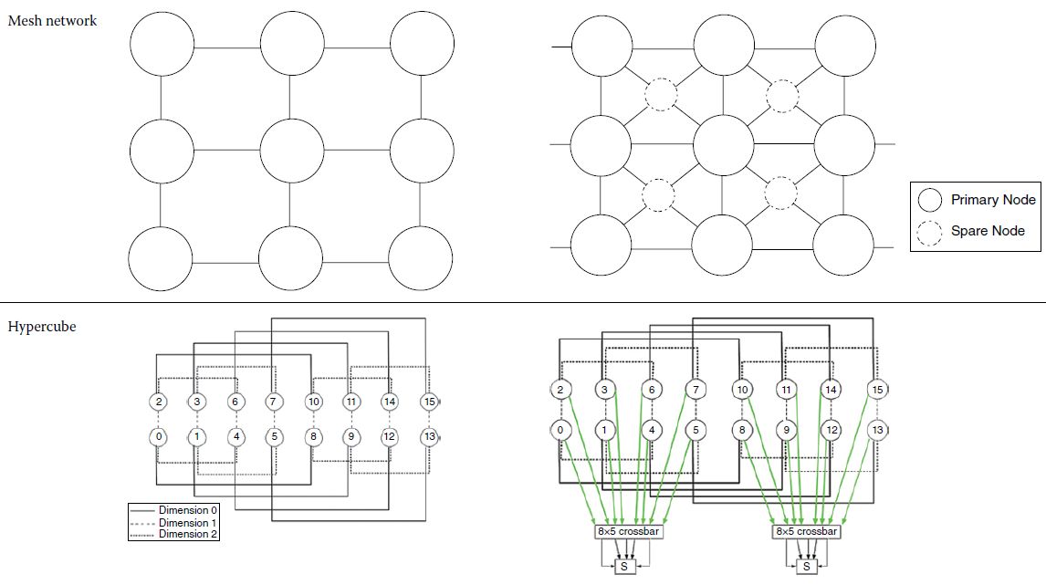
Fault tolerance can be incorporated into a network by having either multiple paths between all source–destination pairs or spare nodes and redundant links that can replace the failed nodes or links. There may be more than one alternative for designing a fault‐tolerant topology, and it can be based on redundant links or spare nodes. Some of the common network topologies and their associated fault‐tolerant topologies [11] are indicated in Table 14.5.

14.2.2 Autonomic Network

Owing to escalation of market requirements and advancement in technologies, there has been a reduction in the time available for development and testing. With every new system being introduced, the complexity of the system in terms of hardware components, interconnections, and lines of code increases, and the size of the smallest building block of the system decreases, going to nanoscale in the present day. This leads to a high probability of inception of faults at some stage or other of network design, configuration, or operation. As the probability of faults increased, the design of network systems went through a paradigm change from being simply fault tolerant to being self‐healing. Systems are being designed to be aware of themselves as well as of their operating environment. An autonomic network system has the capability to continue operation even after fault detection, and also rectifies the fault itself without human intervention. Although most of these features are difficult to incorporate in a wired network, these are common features of present‐day wireless networks in general and of ad hoc and sensor networks in particular.

An autonomic network [22] has self‐configuring, self‐optimizing, self‐managing, self‐protecting, and self‐healing capabilities. A network system, as is common in the case of sensor networks, is self‐configuring if after deployment it discovers its neighbors, detects its environment, becomes aware of the communication requirement, and configures itself not only to be a part of the network but also to continue optimum operation by updating its configuration to support mobility and security. The network systems, being resource constrained with high operational requirement, are also self‐optimizing, reducing power, computation, and bandwidth requirement and increasing the life of the network and its utilization. The self‐protecting feature of the network relates to prevention of network intrusion and security attacks on the network of links in order to ensure availability, integrity, and confidentiality of the network. Further, if the network is compromised or disrupted, the network system possesses the self‐healing capabilities to detect the intrusion and the points of failure and to continue operation from an alternative segment or recover the compromised or damaged links and nodes. An autonomic network system may run through one or more of these capabilities to ensure adaptability and continued operation, as indicated in Figure 14.9.

14.3 Network Management for Fault Detection

Communication networks have acquired increased significance today in the wake of network‐centric operations. Decision‐making in the field by the network devices as well as by the administrator is based on information about resources, node location, and other vital information obtained using the latest means of communication. The need for real‐time and accurate information makes pressing demands on today’s networks. It is important to understand the challenges involved in the management of communication networks and some of the approaches involved in the implementation of management systems for such networks. The use of mobile agent technology as a framework for implementing network management systems is a recent trend. The use of policy‐based network management to delegate management functions and automate decision‐making is also an upcoming area.

Future network application, which may be in disaster management, health monitoring, industrial application, or warfare, envisages rapid engagement in the operational scenario and requires a resilient, high‐capacity backbone extending its reach up to the tactical deployment area. Changes in planning, monitoring, and management in operationally focused tactical communications networks are warranted to match the rapid engagement as well as the advancement in communication technology, which has taken a great leap forward. Advanced network management techniques are now being adopted to manage tactical communication networks.

In this digital‐application field scenario, information holds the key to success. In a battlefield scenario managed either locally or remotely across continents, the commanders and the troops are increasingly becoming dependent on information to execute operations successfully. The dynamics of the tactical requirements and the commander’s intent distinguishes modern tactical networks from commercial networks. These modern tactical networks have constraints in terms of bandwidth and intermittent connections and are subject to changes driven by the commander’s intent, which affects the network behaviors and characteristics and the use of network resources.

14.3.1 Traditional Network Management

Traditional network management systems are based on the manager agent (MA) paradigm. The agent is a software code that resides on the network device and collects management information and sends it to the manager. The manager collects the information from agents, processes it, and generates reports. The interactions between the manager and agent are governed by management protocol. Simple Network Management Protocol (SNMP), standardized by the Internet Engineering Task Force (IETF), is the most commonly used management protocol. It has three versions – SNMP v1, v2, and v3. Some of the other protocols used for network management are netconf, syslog, and net flow. The architecture of a traditional network management system is illustrated in Figure 14.10.

Management functions are often characterized using reference models. The most common reference model is the FCAPS model proposed by IETF. It covers the following management functions:

1. fault management,
2. configuration management,
3. accounting management,
4. performance management,
5. security management.

Traditional network management systems, which are often characterized by a centralized architecture, prove incapable when used in the tactical environment. Management of tactical networks poses several challenges owing to the inherent nature of the operations involved. Some of the challenges are listed below [23]:

• critical response time,
• rapidly changing topology,
• limited resources,
• flexibility.

The periodic polling of the agents by the manager in traditional systems and regular exchange of management information put a strain on the limited bandwidth and add to the delay in transmission and congestion [24]. Owing to these challenges, management of tactical networks calls for a paradigm shift in design and implementation.

14.3.2 Mobile Agent

The MA approach uses a mobile code as an agent instead of a static agent. A single agent now traverses the network and collects management information. This approach significantly reduces the bandwidth consumed for management purposes. It also increases the performance, as only the final result is sent to the manager and most of the processing is done by the MA at the local level. The MA technology has several features that make it promising for use in tactical environments. The decentralization and delegation of management functions ensure that, if a part of the network is compromised, the management of the entire network is not affected.

The architecture of a mobile‐agent‐based tactical network management system is illustrated in Figure 14.11.

The system consists of a mobile agent generator (MAG), which generates MA with the functionality to migrate across the network. The agent traverses the network, collects the management information, processes it, and moves to the next element. The manager controls the movement of the agent, manages its security, and stores the results.

MA technology is now increasingly being used in new implementation strategies to monitor networks. However, there are certain challenges that should be addressed to utilize its full potential. The primary concern in all instances of MA deployment has been security. Given that MAs may traverse hostile tactical networks with classified management information on them, it is imperative to ensure their security. Robust security frameworks have been suggested with advanced authentication and cryptographic techniques [25]. Coordination of agents and prevention of conflicts and deadlocks are among the other challenges that a MA‐based management system has to address.

14.3.3 Policy‐Based Network Management

Policy‐based management is another approach that is being adopted over static management systems in tactical network management. Tactical networks are often complex and heterogeneous, comprising a myriad of components ranging from laptops to management consoles to wireless radios. The topology of such networks is often varying, necessitating the need for adaptive configuration management. Fault management in field networks also requires automation owing to the critical nature of the operations involved. Policy‐based network management systems provide automated response to situations based on predefined policies. The policies are stored in a repository in a policy server. The architecture of a policy‐based network management (PBNM) system is illustrated in Figure 14.12.

The system has the following components [26]:

1. The policy repository is a database of predefined directives that enable the system to take decisions depending on the situation.
2. The policy decision point (PDP) performs the task of choosing the policy from the database depending on the inputs from the clients.
3. The policy enforcement point (PEP) acts as an interface between the PDP and the clients or the network elements.

The communication between the PDP and the PEP is governed by the Common Open Policy Service Protocol (COPS). Policy‐based systems minimize manual intervention and automate most of the functions of network management, thereby facilitating their use in the mission and time‐critical tactical networks.

14.4 Wireless Tactical Networks

Wireless networking has changed the rules of communication, security, and interception in a tactical network. Resourceless communication on the move without any physical footprint is a success factor in today’s scenario. Wireless communication protocols, models, and equipment are available for mobile as well as static users and systems on any platform – aerial, land, water, and even underwater. The range of present‐day wireless networks used in defense applications as well as in civilian applications varies from a few nanometers to submarine–satellite communication. However, the technologies and protocols change with distance. Theoretically, an ad hoc network is generally of higher communication range with better power availability than a wireless sensor network. The rate of data transmission within a similar type of network makes it difficult to standardize any crypto or cryptanalysis engines. For example, a personal area network can be categorized into WPAN, high‐rate WPAN, low‐rate WPAN, mesh networking, and body area networks. Personal area networking, which supports the smart soldier, encompasses the wireless technologies of Bluetooth, Z‐Wave, ZigBee, 6LoWPAN, ISA‐100, RFID, and Wireless HART. The upcoming standards in the field of personal area networks, which are yet to be explored for critical applications, are Internalnet, Skimplex, and Dash7. The key distribution in a wireless network is a challenge in itself, which is yet to be resolved.

The applications of wireless tactical networks are also increasing day by day. Wireless sensor networks and ad hoc networks are technologies of the past. They have graduated to vehicular ad hoc networks (VANETs), underwater sensor networks, and networks within the human body – from sensor‐enabled patients to robotic soldiers and their weapon systems. These scenarios have made the management of wireless networks even tougher because there are deviations in the wireless networks in addition to mobility and localization problems. The nodes can connect to any network at any time and again leave the network. Identifying friend, foe, and captured sensors is a challenge assigned to the network management system.

Transformation of defense forces to meet the threats of fourth‐generation warfare will be heavily dependent on technology as a key enabler and force multiplier. The tactical commander’s aims and objectives of battle and consequent design of battle will be greatly dependent on the flow of information from the digital battlefield. Despite all the technological advancements, the real‐time flow of communication from the tactical battle area is a major concern.

Net‐centric warfare command, communication, computation, information, surveillance, and reconnaissance capability should be improved in order to enhance situational awareness and the capability to identify, monitor, and destroy targets in real time. These activities have to be coordinated, which will further ensure enhanced battlefield transparency at each level of command, leading to responsive decision‐making in near real time. A robust backbone network will therefore act as a force multiplier that will facilitate cumulative employment of destructive power at the most vulnerable point of the enemy.

14.5 Routing in Delay‐Tolerant Networks

The present‐day Internet connects computers across continents over TCP/IP through different types of link providing point‐to‐point connectivity. The Internet was designed to work on symmetric bidirectional links, comparatively low error rates, enough bandwidth for effective data transmission, and short delay between data transmission and data reception.

The evolution of wireless networks added a new variety of network environments over which data communication was to occur. The wireless network has asymmetric links, high error rates due to loss and collisions, intermittent connectivity due to link disruptions and reconnections, higher error rates, and longer and variable delays in data transmission. Examples of such wireless networks are the networks used in network‐centric operations connecting the soldier, combat vehicles, airborne systems, satellites, and surface as well as submerged vessels in the sea. The operating scenario of mobile land networks for civilian usage is no different.

There may be a number of reasons for intermittent connectivity in a network, some well known, including moving out of reception range on account of mobility, node shutdown to preserve power, maintain electromagnetic silence, or preserve secrecy, and configuration for only opportunistic communication or the effect of jamming on the network. Besides the unavailability of the next hop, there may also be long queuing times for messages before delivery. A delay‐tolerant network enables interoperability among heterogeneous networks or Internet buffering of the long delays in communication among them, which otherwise would be a mismatch and hence unacceptable.

References

1. 1 A. Conti, M. Guerra, D. Dardari, N. Decarli, and M. Z. Win. Network experimentation for cooperative localization. IEEE Journal on Selected Areas in Communications, 30(2):467–475, 2012.
2. 2 J. L. Guardado, J. L. Naredo, P. Moreno, and C. R. Fuerte. A comparative study of neural network efficiency in power transformers diagnosis using dissolved gas analysis. IEEE Transactions on Power Delivery, 16:4, 2001.
3. 3 N. O. Sokal and A. D. Sokal. Class E – a new class of high‐efficiency tuned single‐ended switching power amplifiers. IEEE Journal of Solid‐State Circuits, 10(3):168–176, 1975.
4. 4 Y. Han and D. J. Perreault. Analysis and design of high efficiency matching networks. IEEE Transactions on Power Electronics, 21(5):1484–1491, 2006.
5. 5 M. P. van den Heuvel, J. S. Cornelis, R. S. Kahn, and H. E. Hulshoff Pol. Efficiency of functional brain networks and intellectual performance. The Journal of Neuroscience, 29(23):7619–7624, 2009.
6. 6 Network, http://www.webopedia.com/TERM/N/network.html.
7. 7 Computer Network, http://en.wikipedia.org/wiki/Computer_network.
8. 8 A. Avizienis and J. C. Laprie. Dependable computing: from concepts to design diversity. Proceedings of the IEEE, 74, May 1986.
9. 9 P. Jalote. Fault Tolerance in Distributed Systems. PTR Prentice Hall, 1994.
10. 10 M. L. Shooman. Reliability of Computer Systems and Networks: Fault Tolerance, Analysis, and Design. Wiley‐Interscience, 2001.
11. 11 I. Koren and C. M. Krishna. Fault‐Tolerant Systems. Morgan Kaufmann, 2010.
12. 12 C. E. Ebeling. An Introduction to Reliability and Maintainability Engineering. Tata McGraw‐Hill Education, 1997.
13. 13 K. S. Trivedi. Probability and Statistics with Reliability, Queuing, and Computer Science Applications. John Wiley, 2002.
14. 14 S. McLaughlin, P. M. Grant, J. S. Thompson, H. Haas, D. I. Laurenson, C. Khirallah, Y. Hou, and R. Wang. Techniques for improving cellular radio base station energy efficiency. IEEE Wireless Communications, 18(5):10–17, 2011.
15. 15 E. O. Schweitzer III, B. Fleming, T. J. Lee, and P. M. Anderson. Reliability analysis of transmission protection using fault tree methods. 24th Annual Western Protective Relay Conference, pp. 1–17, 1997.
16. 16 T. Korkmaz and K. Sarac. Characterizing link and path reliability in large‐scale wireless sensor networks. IEEE 6th International Conference on Wireless and Mobile Computing, Networking and Communications (WiMob), October 2010.
17. 17 H. Chin‐Yu, M. R. Lyu, and K. Sy‐Yen. A unified scheme of some nonhomogenous Poisson process models for software reliability estimation. IEEE Transactions on Software Engineering, 29(3):261–269, 2003.
18. 18 J. DeMercado, N. Spyratos, and B. A. Bowen. A method for calculation of network reliability. IEEE Transactions on Reliability, R‐25(2):71–76, 1976.
19. 19 Fault Taxonomy. iitkgp.intinno.com/courses/738/wfiles/92209.
20. 20 Electronic Architecture and System Engineering for Integrated Safety Systems (EASIS). http://www.transport‐research.info/Upload/Documents/201007/20100726_144640_68442_EASIS‐.pdf.
21. 21 A. Avizienis, J.‐C. Laprie, B. Randell, and C. Landwehr. Basic concepts and taxonomy of dependable and secure computing. IEEE Transactions on Dependable and Secure Computing, 1(1):11–33, 2004.
22. 22 J. O. Kephart and D. M. Chess. The vision of autonomic computing. Computer, 36(1):41–50, 2003.
23. 23 D. Vergados, J. Soldatos, and E. Vayias. Management architecture in tactical communication networks. 21st Century Military Communications Conference Proceedings MILCOM, Volume 1, pp. 100–104, 2001.
24. 24 F. Guo, B. Zeng, and L. Z. Cui. A distributed network management framework based on mobile agents. 3rd International Conference on Multimedia and Ubiquitous Engineering MUE ’09, June 2009.
25. 25 M. A. M. Ibrahim. Distributed network management with secured mobile agent support. International Conference on Electronics and Information Engineering (ICEIE), Volume 1, pp. V1‐247–V1‐253, 2010.
26. 26 K.‐S. Ok, D. W. Hong, and B. S. Chang. The design of service management system based on policy‐based network management. International Conference on Networking and Services ICNS ’06, pp. 59–64, July 2006.
27. 27 Delay tolerant networking architecture, IETE Trust, RFC 4838. http://tools.ietf.org/html/rfc4838.
28. 28 Bundle Protocol Specification, IETE Trust, RFC 5050. http://tools.ietf.org/html/rfc5050.

Abbreviations/Terminologies

COPS

Common Open Policy Service Protocol

DTN

Delay‐Tolerant Network

HART

Highway Addressable Remote Transducer (Protocol)

IETF

Internet Engineering Task Force

IP

Internet Protocol

LAN

Local Area Network

MA

Mobile Agent

MAG

Mobile Agent Generator

MAN

Metropolitan Area Network

MTBF

Mean Time Between Failures

MTTF

Mean Time to Failure

MTTR

Mean Time to Repair

NIC

Network Interface Card

PBNM

Policy‐Based Network Management

PDP

Policy Decision Point

PEP

Policy Enforcement Point

RFID

Radio Frequency Identification

SCADA

Supervisory Control and Data Acquisition

SNMP

Simple Network Management Protocol

TCP

Transmission Control Protocol

UPS

Uninterrupted Power Supply

VANET

Vehicular ad hoc Network

WAN

Wide Area Network

WPAN

Wireless Personal Area Network

6LoWPAN

IPv6 over Low‐Power Wireless Personal Area Networks

Questions

1. What is software reliability and how do we determine the reliability of software?
2. In the earlier days, systolic arrays were used for fault tolerance. Study about systolic computing and describe the role played by the systolic arrays in fault tolerance.
3. What is autonomic computing and what are the features of an autonomic system?
4. Differentiate between availability and reliability. A network goes down for 1 s every hour. What is the reliability, availability, MTBF, and MTTF for this network over a period of 1 day?
5. Explain the process of reliability calculation using minterms.
6. Describe the three types of fault based on the frequency of reoccurrence of the fault.
7. Explain the difference between a fail silent system and a gracefully degraded system. Mention a scenario of application for each where a fail silent system will be required and a gracefully degraded system cannot work, and vice versa.
8. Draw various fault‐tolerant network architectures and their equivalent non‐fault‐tolerant designs.
9. Describe the working of a mobile agent.
10. Explain the policy‐based network management approach.
11. Why are delay‐tolerant networks required? Justify your answer giving examples.
12. Explain the working of a bundle protocol.
13. There can be a number of reasons, other than security attacks or battery failure, for link disruptions and intermittent connectivity between wireless nodes. Mention a few such reasons.
14. State whether the following statements are true or false and give reasons for the answer
    1. Reliability is the average time over a given period when the system is operational.
    2. For a network that goes down very frequently, reliability and availability are the same.
    3. MTTF = MTBF − MTTR.
    4. If F(t) is the probability that a component will fail at or before time t, and λ(t) is the failure rate of the component at time t, then F(t) = 1 − e^–λt.
    5. If a transient fault occurs in the network, the network goes down for a long period until it is repaired and made operational manually.
    6. A fail silent system does not stop working immediately on detection of a fault, but keeps working with lower performance for a very long period and then silently goes down.
    7. In a policy‐based network management, PDP acts as an interface with the clients or the network elements.
    8. Bluetooth, Z‐Wave, ZigBee, 6LoWPAN, ISA‐100, and RFID are wireless technologies.
    9. Internalnet, Skimplex, and Dash7 are security standards.
    10. Bundle protocol is a routing protocol used in delay‐tolerant networks.

Exercises

1. Calculate the reliability of communication between points A and B of the network given below. The reliability of each communication link is indicated with each of the links.

   

2. A certain cryptographic system uses a shared key. The key is spread across four different smart cards, and all the smart cards are required to decrypt the information. All the smart cards are similar and the reliability of a smart card is 0.7 What is the reliability of the information being decrypted? What will the new reliability be if USB crypto tokens with a reliability of 0.9 are used in place of smart cards?
3. A data center is said to have an availability of four 9s if it has an availability of 99.99%, five 9s if it has an availability of 99.999%, and so on. What is the permissible downtime per year permitted in data centers with two 9s (99%), three 9s, four 9s, five 9s, and six 9s?
4. A data center provides power to the servers through its uninterrupted power supplies (UPSs), and each UPS has a reliability of 99%. The designers of the data center want to provide power to the servers with a reliability of 99.671%. A minimum of how many UPSs have to be placed in parallel to ensure this reliability. By how many does the number of UPSs in parallel have to be increased at each stage if the designers plan to increase the reliability in stages to 99.741% and then to 99.982% and then finally to 99.995%?
5. A network is depicted below as a probabilistic graph. Calculate the reliability of the network using minterms for communication between X and Y.