10
Routing in Wireless Ad Hoc Networks
10.1 Introduction
Gordon Moore, who was the cofounder of Intel, predicted ‘Transistor density of minimum‐cost semiconductor chips would double roughly every 18 months’. The prediction was made in 1965 and it has been more than five decades since then, but still the predicted trend holds its ground. This has led to its being called Moore’s law. The density of transistors is directly related to the processing speed and inversely related to the cost of the microprocessor. The effect of Moore’s law is that the performance of a processor is doubling up every 2 years, and the capacity of memory for the same covered area doubles up every 18 months. This has led to miniaturization of the computers and other computing systems over the past few years, as well as reduction in their cost. The advancements in microprocessor and computing technology have made available laptops, mobile phones, and iPADs at affordable cost at the grassroots level. This has led to the application of computing systems in all imaginable applications, scenarios, and geographic domains.
The size of the modern day computing device and its application has provided mobility to these devices. The ease of operations, fast deployment possibility, freedom from wired mesh, and support for mobility have led to invention and advancements in the field of wireless technology, and the area is growing rapidly [1, 2]. The wireless mode of communication between two nodes, either mobile or static, can be supported by two different methodologies:
- infrastructure‐based mobile wireless communication, i.e. a wireless cellular network;
- infrastructureless mobile wireless communication, i.e. a wireless ad hoc network.
The difference between a wireless cellular network and a wireless ad hoc network has been tabulated in Table 10.1.
Table 10.1 Comparison of a cellular wireless network and an ad hoc wireless network.
| Comparison Parameter | Cellular Wireless Network | Ad Hoc Wireless Network |
| Centralized infrastructure and management | Required. | Not required. |
| Time for setup | High. | Low. |
| Networking cost | High. | Low. |
| Network designing and planning | Required for establishing the base stations. | Little or even not required. |
| Reliability and stability | Comparatively higher than an ad hoc network. | Comparatively lower than a cellular network. |
| Resource constraint | The nodes might have resource constraint, but the routers and access points have sufficient resources. | The nodes act as hosts as well as routing devices, and hence resource constraint. |
| Reachability | The range of communication is pre‐fixed. The network can be operational only at those locations where the cellular infrastructure exists. | New nodes can automatically be connected to the network, changing the range of connectivity. The network can be made operational at any place, including underwater, above the land, or in the sky. |
| Range of communication and connectivity | The range may even extend to communication connectivity across a country. | The spread of the network is generally confined to its application theater, which may be limited to an operational area, building, campus, or a very small geographic region for some specific defense or civilian application. |
| Topology | The topology of the backbone is static. | The entire network topology is dynamic. |
An ad hoc network is made on‐the‐fly by the participating nodes without requirement of any centralized infrastructure. ‘Ad hoc’ is a Latin phrase that means ‘for this’, and this phrase defines well the characteristic of an ad hoc network, which is created by its participating nodes for this (any) particular application [3]. An ad hoc network is formed by two or more participating nodes that want to communicate with each other and do not possess the time, resource, or scenario to set up a traditional network in terms of wired connectivity or routing and administrative infrastructures in terms of access points, switches, and routers. The nodes in an ad hoc network may communicate continuously, regularly, or on a requirement basis. The lack of network support infrastructure necessitates the participating network nodes of the ad hoc network to help each other in communicating in the network. This makes them play the dual role of host as well as the networking device. The ‘network device’ role of the node is responsible for one or more of the activities such as signal amplification, packet forwarding, detecting neighbor nodes, participating in routing, detecting network attacks, and ensuring secured communication. The reach or the size of an ad hoc network completely depends on the number of participating nodes, as well as the willingness of these ad hoc nodes to participate in the process of routing information to and from their neighbors.
The precursor of the ad hoc network [4] was the packet radio network (PRNET) designed and developed by the US Department of Defence (DoD). The research on the packet radio network was initiated in 1972 to provide reliable communication between computers for military applications. The PRNET, which used ALOHA and Carrier Sense Multiple Access (CSMA) protocols, was continuously improved during the period 1973–1987 when a number of network devices and protocols came up to improve the network. The PRNET used radio frequency to provide half‐duplex communication at 100 and 400 kbps. In the early 1980s, the survivable adaptive radio network (SURAN) evolved to support networking between battlefield equipment, platforms, and soldiers in a mobile, infrastructureless, and hostile terrain. SURAN provided packet switching over improved radios, which were smaller and cheaper. The PRNET used a distance vector algorithm, while SURAN was based on a hierarchical link state algorithm. The era of PRNET is called the ‘first generation’ of ad hoc networks, while SURAN initiated the beginning of the ‘second generation’ of ad hoc networks, which continued until 1993.
The second generation of ad hoc networks also saw the advent of global mobile (GloMo) information systems and near‐term digital radio (NTDR) systems from DARPA. The GloMo information system used flat as well hierarchical routing algorithms and brought in the concept of self‐configuring and self‐healing networks. The GloMo network was meant mainly for providing anytime‐anywhere access to multimedia‐based defense information systems in the hand‐held devices of the mobile forces under deployment. The NTDR was a self‐organizing and self‐healing radio network based on clustering and link state routing that was used to provide connectivity at a brigade level of the defense forces. A brigade comprises 3–5 regiments. Each regiment has about a thousand soldiers, along with small and medium arms, equipment, guns, vehicles – tracked or wheeled or other platforms such as armored vehicles, depending on the role and formation of the regiment. NTDR had a two‐tier architecture and was meant to provide data communication between the brigade‐level command and control center and the regiment and other formations further in the regiment.
The third generation of ad hoc networks marked its beginning from 1990 and saw a shift in ad hoc network applications from defense use to commercial applications. Miniaturization of computers led to the invention of laptops and notebooks and the introduction of 802.11 PCMCI cards enhancing mobility. Research in the area of ad hoc networks gained momentum in the academic institutes during this period. IETF created the MANET working group. Bluetooth, HIPERLAN, and mobile ad hoc sensor networks were also introduced in this period.
10.1.1 Basics of Wireless Ad Hoc Networks
The nodes participating in the creation of a wireless ad hoc network should possess a network adapter capable of wireless communication. The nodes may be mobile or static. There are certain special types of node in an ad hoc network that are generally static, e.g. access points, which may provide connectivity between the ad hoc network and the Internet or some other backbone network, either wired or wireless. Two nodes in a wireless ad hoc network can communicate only if they are in the direct transmission range and reception range of each other. They can also communicate with each other through one or more intermediate nodes if routing of packets from the source to the destination is allowed through the intermediate nodes. Hence, the source node as well as the destination node should individually have an overlapping transmission and reception region with at least one intermediate node each nearer to it. Each of the intermediate routing nodes should also have an overlapping reception–transmission region with at least two other intermediate node or source node or destination node as indicated in Figure 10.1.

Figure 10.1 Basic wireless ad hoc network.
As can be understood from Figure 10.1, ad hoc networks are also capable of forming multiple paths between a particular source and destination pair. Furthermore, as there is no centralized node for managing or administrating the network, there is no single point of failure. This leads to enhancement of the reliability and fault tolerance of a wireless ad hoc network. There are frequent topological changes in an ad hoc network because the nodes are mobile, toggle between sleep mode and active mode, come into the transmission zone, or move out of it. The routing protocols for an ad hoc network are designed to accommodate these basic characteristics of the network. These routing protocols accommodate topological changes not only due to movement of nodes but also due to frequent link disruptions and new link availability. The link instability is due to sudden availability or non‐availability of intermediate nodes for routing. The wireless nature of an ad hoc network further enhances the need for such routing protocols, as the nodes are free from the constraint of limited or restricted mobility as in wired networks.
The nodes participating in the formation of a wireless ad hoc network can be laptops, mobile phones, smart phones, personal digital assistants, and any other ad‐hoc‐network‐enabled device used in applications for defense, health, industry, home, or transportation. The main characteristic of an ad hoc network, which has opened up the entire spectrum of its application, is that the network is ‘infrastructureless’. Hence, it is the most preferred type of network in a disaster‐hit area. A disaster, natural or man induced, e.g. an earthquake, flash floods, landslides, a tsunami, an avalanche, explosions, or a fire, may wipe off all the available network infrastructure, rendering the wired communication as well as the wireless cellular communication inactive. In such scenarios, an ad hoc network is the cheapest and fastest way to set up a communication network for information exchange among the participating nodes. The network provides sufficient bandwidth and is established immediately on demand and is reliable. Similar requirements also exist in the case of events that lead to a sudden influx of people in a particular region that may not have any prior networking infrastructure or may lack sufficient infrastructure to cater for a sudden increase in node connectivity requirement. These events may be a collection of people at conferences, jamborees, carnivals, melas, exhibitions, trials, and cross‐country events, or defense applications such as fleet reviews and land or offshore exercises, or some political event leading to a mass exodus of citizens. In the case of these scenarios, an ad hoc network can help to set up, without exploiting any pre‐existing network infrastructure available in the region, communication between the enabled devices held by the people.
Ad hoc networks are designed to be self‐configuring, self‐organizing, and self‐healing in nature [5]. The nodes in them are able not only to interconnect with each other but also to continue to retain their connectivity by adapting to various changing parameters in the network, including variation in signal strength, changing mobility rate, variation in topology of nodes, node failure, or link failure. They discover their neighbors on booting up, and thereafter they are capable of computing the route from themselves to every other connected node in the network and selecting the optimum route. The optimum route can be in terms of number of hops, total energy consumption, number of packets transmitted, or control messages exchanged.
A node in an ad hoc network collaborates with the neighboring nodes to identify the network and continuously adapts to the changing network parameters to route data packets to the destination. The node shares with all its neighboring nodes on a continuous or on‐demand basis the information gathered relating to its neighbor connectivity, network topology, and route to destination nodes using multihop over other intermediate nodes. This enables all the nodes to self‐heal themselves to the changing network with the help of a routing algorithm being run by it. This characteristic of the ad hoc network is also called ‘fault tolerance’.
The network architecture, routing capabilities, and operational requirements of an ad hoc network lead to the possession of the following characteristics by a wireless ad hoc network:
- Distributed processing across nodes for path determination and packet forwarding.
- Variation in network topology and number of nodes.
- Dynamic topology due to mobility of nodes.
- Energy constrained, low power nodes.
- Unreliable links and variable link capacity.
- Heterogeneous link characteristics such as unidirectional links, omnidirectional links, and point‐to‐point links.
- Capability of neighbor discovery for peer‐to‐peer routing.
- Autonomous mode of operation by each node owing to lack of a centralized administrator or management.
- Self‐configuring and self‐healing.
In an ad hoc network, a link may be unidirectional not only because of its manufacturing or configuration setting but also because of a number of other operational, environmental, or technical factors. A few factors that lead to unidirectional behavior of the links are as follows [6]:
- The reception hardware and the transmitting radio may not be of equal power and range in the node.
- A node may decide to maintain electromagnetic silence owing to some operational threat in the area or to protect itself from being detected in an enemy territory. In such a scenario, the node, even though capable of bidirectional communication, will use a unidirectional link only to listen to the network transmissions or receive packets from the network and impede its ability of packet transmission.
- The toggling between bidirectional and unidirectional states of the link may vary with time owing to environmental effects and traffic parameters.
- The link in any one direction may become unavailable owing to heavy signal interference around one of the nodes. The node density may be very high around one of the nodes, reducing channel availability towards this node from some other node. A node willing to transmit may be from a less dense area and waiting very long to transmit data to a node in a dense area. The waiting period may be long enough effectively to make it an unavailable transmission link and turn it into a unidirectional link. A scenario depicting this situation can be understood from Figure 10.2. Node 1 wants to transmit a packet to node 2. However, as node 2 has a huge number of active nodes in its reception range, which may be involved in packet exchange, node 2 may not be able to receive a data packet from node 1. Contrary to this, whenever node 2 wants to send a packet to node 1, it can do so with relative ease as there will be no interference around node 1.

Figure 10.2 Unavailable node due to high interference.
The hidden terminal problem and exposed terminal problem are also two typical technical issues faced in a wireless network, and hence solutions for them have to exist in mobile ad hoc networks. Hidden nodes, with respect to a particular node or a collection of ‘N’ nodes in a wireless network, refer to the set of nodes that are outside the range of ‘N’. To present the problem in a simple manner, consider three nodes, node 1, node 2, and node 3, such that node 1 is in the range of node 2 as well as node 3, but node 2 is not in the range of node 3, as depicted in Figure 10.3. Hence, node 1 can transmit to (referred to as ‘see’) node 2 and node 3, but node 2 cannot see node 3, and vice versa. Now, at a particular instant of time ‘t’, node 2 plans to communicate with node 1, and so it senses the wireless medium, does not detect any interference, and therefore transmits. At the same time instant ‘t’, node 3 also plans to communicate with node 1, senses the wireless channel to be free, and thus transmits. In this particular scenario, Carrier Sense Multiple Access/Collision Avoidance (CSMA/CA) also fails to work. This leads to collision of signals at node 1, leading to loss of data, and node 1 does not receive any transmission either from node 2 or from node 3. This is referred to as the hidden terminal problem.
Figure 10.3 Hidden node.
The hidden terminal problem is resolved by reserving the channel and notifying others before transmission of data, as depicted in Figure 10.4. Node 2 sends a ‘request to send’ (RTS) to node 1 that it is willing to transmit. On receiving the RTS signal from node 2, node 1 sends a short frame to its neighbors to indicate that shortly a transmission involving node 1 will occur, a ‘clear to send’ (CTS) signal is sent to node 2, and thus the channel is presumed to be reserved as the neighbors restrain from transmission until the channel passes off a large frame. The RTS/CTS signaling works only in those cases where the packets to be transmitted are relatively larger than the RTS/CTS packet size. If the packet to be transmitted from one node to another node is comparable with the packet size of RTS/CTS, the packet is transmitted directly over the wireless channel without invoking RTS/CTS signaling to reduce time and complexity. Furthermore, RTS packets from node 2 and node 3 can also collide. Hence, an optimization has to be done for using RTS/CTS signaling, and the threshold level has to be determined to invoke it.

Figure 10.4 Resolving the hidden node problem.
The solution to the hidden node problem leads to another problem, the ‘exposed node’ problem, which can be understood from the same example as in Figure 10.3 but with another node, node 4, added to the network, as depicted in Figure 10.5, such that node 4 is in the range of node 3 but is not in the range of node 1 or node 2. Now, if node 1 is communicating with node 2 and at the same time node 4 wants to communicate with node 3, this cannot be done because node 3 will not grant a CTS signal to node 4 because node 3 has already received a short frame from node 2 and hence assumes that it cannot send a clear signal to node 4, even though the point‐to‐point communication between node 1 and node 2 and between node 3 and node 4 could happen simultaneously. If such a transmission were permitted, none of the nodes would face any collision as the area of collision would be in the region between node 2 and node 3.

Figure 10.5 The problem of an exposed node.
The typical characteristics of an ad hoc network raises a number of challenges in successful and efficient routing of packets between any two nodes. The dynamic topology leads to a time‐dependent change in the optimal path between any two nodes. The major technical challenges faced in ad hoc routing are listed below:
- Communication channel related – hidden terminal problem, exposed terminal problem, signal fading effect, low bandwidth, packet loss, variation in channel quality, environmental effects.
- Data traffic related – variation in traffic characteristics and profile.
- Device related – heterogeneous nodes, limited wireless range, unidirectional communication, i.e. either receiving or sending in certain nodes, mobility of nodes, variation in mobility pattern and speed, dual role of host as well as intermediate routing device.
- Power related – constrained battery power, power planning, and rationing cannot be done owing to unpredictable packet forwarding requirements.
Based on the interconnectivity among various independent wireless ad hoc networks, these networks are classified [7, 8] into two categories:
- closed mobile ad hoc network,
- open mobile ad hoc network.
In a closed mobile ad hoc network, all the nodes belong to the same network, and hence the nodes participate in networking to cater for the same application. As the nodes belong to the same network, there is a high probability that the nodes are homogeneous. These nodes do not communicate either with any other mobile ad hoc network or with any other type of network such as a cellular network or wired network. All the neighbor discovery, route determination, and packet forwarding are confined within the network, and there is no exchange of information with other networks. These networks lack gateways for connectivity to other networks, as shown in Figure 10.6.
Figure 10.6 Closed ad hoc network.
An open mobile ad hoc network, as shown in Figure 10.7, is formed by interlinking of different mobile ad hoc networks. They are also capable of communicating with other types of network, i.e. a cellular network, a sensor network, and a wired network, through gateways available in the open mobile ad hoc networks. As the network is formed by different types of participating mobile ad hoc network, there may be different types of node in the networks, leading to a high degree of heterogeneity of nodes in the network.

Figure 10.7 Open ad hoc networks.
A closed mobile ad hoc network is generally formed for accomplishment of a single mission by an identified and known group of participating nodes. The mission accomplishment holds priority in the routing over resource conservation in the network. An ad hoc network of laptops formed by a group of researchers conducting a soil study in a desert, an ad hoc network of mobile phones of rescuers to share location and mobility information among each other at a disaster site, an ad hoc network formed among radars for surveillance of a designated area – these are examples of closed mobile ad hoc networks.
In an open ad hoc network, different mobile ad hoc networks, each with its own mission objective, collaborate with each other for resource sharing in terms of packet forwarding to a large extent and information exchange to a lesser extent. As different networks collaborate with each other, this leads to an increase in the spread of the network. The transmission and reception range of the network can increase many fold as intermediate nodes from other networks contribute to packet forwarding, enhancing the transmission range.
As shown in Figure 10.7, some of the participating networks may be located at the periphery of the network, while a few may be located in the central region of the network connecting the networks at the periphery. There might even be networks that have a wider spread and have nodes across the entire open ad hoc network. The nodes in the central region of the network receive more requests for packet forwarding, as they bridge the nodes at the periphery and are in the routing path of most of the source destination pairs. These nodes will therefore consume more resources in terms of processing power and wireless transmission, and hence consume their battery at a faster pace. As each node will attempt to maximize its benefit by participating in the open network, this might lead to selfish behavior by the node.
Each node attempts to use its resource optimally by ensuring its availability for information detection and forwarding related to its own mission. It also attempts to restrict its resource usage when it participates in the packet forwarding related to the mission of some other network forming a part of the open network. The most common example of selfish behavior by a node is that it does not participate in packet forwarding for other participating nodes to save its own battery power consumed for processing the packet and forwarding it, as transmission consumes considerable power in an ad hoc node.
The ad hoc network has a variety of applications and various deployment scenarios. The same routing protocol will not be able to cater for different ad hoc network requirements. Hence, there exist a number of routing protocols, each optimizing one or more parameters on the basis of the priority of the requirements. Still, new routing protocols are evolving to cater for the changing requirements and improving the existing algorithms. A single protocol cannot have all the functionalities optimizing all the parameters required in different scenarios, as they may be complementary to each other. A cumulative list of properties [3, 9‐11] that should be considered before designing or analyzing a routing protocol is given below:
- The protocol should be able to do multicasting, i.e. send packets from one node to multiple nodes simultaneously. The property of multicasting should not be assumed to be present if the protocol has the capability of broadcasting packets. Multicasting consumes less resources than broadcasting.
- The protocol should converge rapidly in the dynamic network topology.
- The protocol should be highly scalable, enabling it to connect to a large number of nodes that may even be heterogeneous.
- The protocol should be small and simple for reduced memory requirements and ease of path prediction and performance analysis.
- The protocol should discover a loop‐free path, i.e. it should not visit the same link twice unless the network has been reconfigured while the data packet was in transit, leading to changes in the routing table of intermediate nodes, necessitating a revisit to particular links.
- To recover from link failures and congestion avoidance and to save time spent rediscovering routes in the case of some change in network topology, the routing protocol should discover redundant paths from source to destination before transmission of packets.
- The protocol should avoid a single point of failure in terms of its presence in a single node for any administrative, management, or control function. The protocol should be distributed in nature, so that it is unaffected in the case of any random failure of nodes.
- The protocol should be capable of effective link utilization. The ad hoc network can have unidirectional as well as bidirectional links. The protocol should not be designed to support only one kind of link for particular operations or in a particular region of the network.
- The routing protocol should be designed to minimize resource consumption in terms of processing, channel utilization, and exchange of packets, as all these lead to power consumption, which can be the most constrained resource in an ad hoc network during its usage in certain application scenarios.
- The protocol should be adaptive to misbehaving nodes, sleeping nodes, and captured nodes, as these may lead to unpredictable behavior.
- The protocol should be secure. It should be able to avoid eavesdropping, snooping, disruptions, modifications, repudiation, and cryptanalysis.
10.1.2 Issues with Existing Protocols
The characteristics that make an ad hoc network different from the traditional networks lead to a different set of requirements in wireless ad hoc routing protocols [3]. Mobility is the prime factor driving the wireless ad hoc protocols. The distance as well as the orientation of the nodes may keep changing. To make it further complex, the rate of change in the distance and orientation may also vary. These complexities are then driven by the typical behavior of an ad hoc network, such as processing limitation, power constraint, bandwidth restriction, heterogeneity of the nodes, high scalability, change in the transmission and reception range of a node due to variation in climatic condition, or variation in the number and distance of neighbor nodes. It is not only these characteristics of the ad hoc nodes that drive the routing protocol, but also unpredictable behavior of the participating nodes, such as selfish behavior, byzantine or captured nodes, sleep nodes, and dumb nodes, which makes the ad hoc routing protocol one of the most researched areas for enhancements and improvements.
In order to effectively handle the ad hoc networking characteristics and constraints, the routing protocol should be highly scalable, adaptive to rapidly changing topology, demand low processing capacity, generate least traffic, and save battery power. However, all these routing characteristics may not be required simultaneously by all types of ad hoc network. Each ad hoc network will require one or more of these routing characteristics, based on the devices used, the application, and the deployment scenario.
An ad hoc network of vehicles on a highway will require the routing protocol to handle high mobility, but it will not be constrained in terms of power owing to the uninterrupted and sufficient availability of battery power from the vehicle. A different scenario would be an ad hoc network of laptops and mobile phones of delegates in a conference hall where scalability of the network will be of utmost concern for the network. Mobility and power conservation may not be the driving characteristics in their routing protocol. Another scenario is the ad hoc network formed by buoys floating in the sea for regular measurement of the oceanographic and sea conditions and processing of the data for weather prediction. In such a network, power saving will be of prime concern, failing which there will be a frequent requirement to retrieve the buoys to change the power source. The power constraint will automatically govern constraints over processor requirement, frequency of transmission, periodicity of updates, and minimization of control traffic. However, in this deployment, mobility is of less concern and scalability will rarely come into play for a particular deployment. Hence, a single routing protocol cannot cater for all the types of ad hoc network.
A particular ad hoc routing protocol that performs best in a particular deployment scenario may not be able to perform optimally in a number of other deployment scenarios. Hence, there are a variety of ad hoc routing protocols, each having its own advantages, disadvantages, and specific application scenario, and each performing optimally only if used after an intelligent judgment.
A routing protocol is designed with two prime objectives – discovery of optimum routes between all source–destination pairs and efficient delivery of packets between any source–destination pair. The objective of the routing protocol remains the same for the conventional routing protocols as well as the routing protocols required for wireless ad hoc networks. Still, there are problems in porting the routing protocols used in wired networks directly to wireless ad hoc networks [3, 12]. The following are the major problems:
- Protocol convergence. The conventional protocols were designed for fixed network topology. As the topology of an ad hoc network is dynamic, it becomes difficult for the conventional protocols to converge.
- Route discovery. The conventional protocols were designed to have a complete view of the network and discover routes for all source–destination pairs. This leads to a high volume of data exchange between the nodes in the form of control signals, which is not acceptable for an ad hoc network as it is resource constrained. Furthermore, in an ad hoc network it is not necessary for each node to know the details of the entire network, and nor does an ad hoc network necessitate the discovery of all source–destination pairs.
- Link characteristics. The conventional protocols were designed for bidirectional links, which were assumed to be reliable in terms of QoS, while in ad hoc networks, not only may the links be unidirectional, they may be turned on and off by the intermediate nodes, and the link parameters are dynamic and unpredictable owing to environmental effects.
- Unusable class of protocols. The conventional protocols can be differentiated into certain categories, and there are particular categories that are downright unsuitable for direct porting from static wired networks to mobile ad hoc networks [13, 14]. A few such categories are as follows:
- Centralized routing protocol. There is a class of conventional protocols that are based on centralized routing where the route discovery is made by a single node in the network. This is not an acceptable practice in ad hoc networks. This therefore renders the entire class of conventional centralized routing protocols in their existing form unusable in ad hoc networks.
- Static routing protocol. The class of static routing protocols for conventional networks is ineffective in its existing form in ad hoc networks with node mobility and dynamic topology.
- Multicast routing protocols. The traditional multicast routing protocols, which are based on source of origin and reverse path forwarding, are not able to perform in the mobile ad hoc environment as the source node may move to a new position after transmitting the packet, rendering the routing protocol ineffective and inefficient. The movement of nodes that are members of a multicast group and the formation of a transient loop during reconfiguration of the spanning tree are two other problem areas when using conventional multicast routing protocols.
10.2 Table‐Driven (Proactive) Routing Protocols
The table‐driven protocols are the family of ad hoc network routing protocols that are closest to wired routing protocols, as most of the algorithms are inherited from the wired network with least variation to fit into the wireless community. Proactive routing protocols keep the network nodes ready for routing the packets from source to destination. The proactive routing protocols are also known as table‐driven protocols, as they maintain in the nodes a routing table with information about connectivity to other nodes in the network. The routing table is regularly updated through topology information exchange between neighboring nodes with the intention to maintain the route information for every other node in the network. The advantage of this class of protocol is that the shortest distance between any source–destination pair can be found in the least time. Another common name given to the class of table‐driven routing protocols is ‘global’ routing protocols, as the nodes have global (complete) information about the entire network.
Traditionally, the proactive routing protocols are classified into two categories – distance‐vector‐based protocols and link‐state‐based protocols. In distance‐vector‐based proactive routing, each node maintains a routing table that has two major pieces of information – the distance to each node and the next hop node through which the packet should be forwarded to that node. To maintain an updated distance vector table, each node periodically sends its distance vector table to all its neighboring nodes. A node, on receiving a table from its neighboring node, matches the entries in the received table with its own entries. If it finds that the distance to any node is less through its neighbor, then the distance already available in it for that particular destination node is decreased accordingly and the route to that destination node is made via this particular neighboring node from which it received the updated table. The protocol also effectively supports loop avoidance, neighbor discovery, and changes in network topology, though not at a rapid rate.
In the link‐state‐based routing protocol, each node in the network maintains complete information about the network topology. This information is in terms of which node is connected to which other nodes and the condition of the links among them. To maintain updated information, each node regularly broadcasts the status of its links to its neighbors. Dijkstra’s algorithm is generally used by a node to create the routing table. Each node can independently calculate the best path from itself to all other nodes in the network, as they all possess the link state information of the network.
The disadvantages of the table‐driven proactive routing protocol are as follows:
- As the routing table is regularly updated, the resource utilization in terms of bandwidth, processing power, memory, and battery consumption is high.
- The scalability is less, as the routing table stored in each node becomes too large to store and maintain. Furthermore, as all nodes broadcast information, this leads to congestion and interference.
- This routing protocol reacts slowly to the dynamic network topology and may lead to routing failures in the case of rapid node movements.
- There may be certain routes over which no data packet has travelled and also by which there is a high probability that no packet will travel in the future. Still, the protocol utilizes resources to establish and regularly update such paths.
A few table‐driven proactive routing protocols are listed below:
- Ad Hoc Wireless Distribution Service (AWDS),
- BABEL,
- Better Approach to Mobile Ad Hoc Networking (BATMAN),
- Clusterhead Gateway Switch Routing Protocol (CGSR),
- Destination Sequence Distance Vector (DSDV),
- Direction Forward Routing (DFR),
- Distributed Bellman–Ford Routing Protocol (DBF),
- Fisheye State Routing (FSR),
- Hierarchical State Routing Protocol (HSR),
- Optimized Link State Routing Protocol (OLSR),
- Wireless Routing Protocol (WRP).
10.3 On‐Demand (Reactive) Routing Protocols
In a reactive ad hoc routing protocol, the path from a source to a destination is determined when a packet is to be routed between the source–destination pair. As the path is determined on a requirement basis, it is also known as ‘on‐demand’ routing. This routing strategy reduces the routine bandwidth utilization by avoiding exchange of update information between the nodes. However, it adds to the delay in routing a packet to the destination as the path to the destination has to be determined before the packet can be routed. This routing strategy is effective in the case of large networks with relatively stable nodes, as the strategy adapts well to a dynamic network. Hence, the performance of a proactive routing protocol as well as a reactive routing protocol depends on the size of the network, the mobility of the nodes, and the frequency of communication between the nodes, and one routing protocol will perform better than another, depending on these parameters.
The source node initiates the process of route discovery when it is required to forward a packet to a destination. The family of reactive protocols generally relies on a variety of classical flooding algorithms and their improvements for route discovery. The reactive routing protocol has two primary operations to perform – route discovery and thereafter maintenance of the discovered routes. Dynamic Source Routing (DSR) is one of the initial on‐demand routing protocols that is explained here with an example in Figure 10.8 to give an overview of an on‐demand routing protocol.


Figure 10.8 Sequence of steps in dynamic source routing.
In a network running DSR [3], the source node embeds in the header of the packet the entire route in terms of the hopping sequence on intermediate nodes before forwarding the packet towards the destination. If the source node (SN) is not aware of the path to the destination node (DN), then SN initiates route discovery. SN broadcasts a route request (RREQ). Each intermediate node (IN), when it detects that it is not the DN for the RREQ, adds its identifier before forwarding the RREQ further. These added identifiers of the INs build up the required hop sequence. The IN forwards the RREQ only if it finds that the route to the DN is not available in its route cache, otherwise it sends a route reply (RREP) back to the SN through the same hop of intermediate nodes through which this IN received the RREQ. As the RREQ already contains the list of node identifiers through which it came, the RREP need not be flooded, but it is unicast back.
The network may not have any INs with information of the route to the DN in its route cache or the RREQ may reach the desired DN before reaching any IN that has the cached route to the DN. When the DN detects that the RREQ is meant for it, it sends back the RREP in a similar way to the IN with the cached route would have done. To reduce flooding of the RREQ, any node before broadcasting the RREQ sends the RREQ to its neighbor with an instruction not to broadcast it and return back the route information if it has the route to the DN in its cached route. If the neighbors do not possess the information, then only the broadcast mode is opted. A node may also operate in promiscuous mode to receive all the packets and use the header information in the packet to gain information about the source route it is carrying.
An RREP can be sent back through the same route from which the RREQ packet came if all the links are bidirectional. If some of the intermediate links are not bidirectional, the RREP may rely on the route cache of the nodes to get the path back to the SN. Alternatively, the RREP is piggybacked on a RREQ packet and the route back to the SN from the DN is again discovered.
The reactive routing strategy also has the task to maintain the discovered route. A route once detected by the source towards the destination may not be available for the entire time duration required to transmit the complete data available at the source to the particular destination. Some of the intermediate nodes in the selected routing path may move out of the transmission range or may run out of energy. These missing intermediate nodes leading to failed links can be detected actively or passively. Active detection is by receiving back acknowledgement from all the previous hops. In passive detection, each node in the routing path listens to its neighbor by entering into promiscuous mode. Information about any detected link failure is transmitted back up to the source node. All the intermediate nodes also learn about this node failure and truncate the path beyond the failed node.
During the process of route discovery from source to destination, the intermediate nodes involved in the route discovery process also learn a number of routes, which each of the nodes stores in its route cache. The source node in the course of discovering the destination node learns about the path to all other intermediate nodes that are on the path to the destination. All the intermediate nodes that receive an RREQ packet from the source learn the path from themselves to the source as well as from themselves to all the other intermediate nodes on the path to the source node. Similarly, the RREP packet makes all the intermediate nodes aware of the route to the destination node and to all the intermediate nodes up to the destination node. The nodes also learn paths while forwarding error messages related to node failure. A node may also operate in promiscuous mode, learning new routes. Thus, reactive routing is associated with a number of opportunities through which the nodes learn about routes to a number of other nodes during the process without initiating any new process specifically for route discovery. The routes learned in this process are stored in the route cache of the nodes, which they use to help other nodes in faster route discovery.
Advantages. The major advantages of the reactive routing protocol are as follows:
- The reactive routing strategy is bandwidth savvy as it not only initiates route discovery on demand but also searches by an incremental method, stopping with the discovery of the destination node.
- Multiple routes are traced from the source to the destination during the process of route discovery. This is due to fresh route discovery as well as replies from intermediate nodes aware of the destination through locally cached route information.
- During the process of route discovery from source to destination, the source also gains information about the routes to the intermediate nodes. The intermediate nodes involved in the process of node discovery also learn about the routes to the source, destination, and intermediate nodes involved in the route discovery.
- There will be certain routes in the network that will never be discovered by the routing strategy. Only those routes through which a packet can possibly be routed efficiently will be discovered.
- Caching of route information by the participating nodes reduces resource utilization during route discovery.
Disadvantages. Some disadvantages of the reactive routing protocol are as follows:
- When a path to a destination has to be determined, generally flooding is used so as to speed up the route discovery process. This results in congestion and collision in the network and also enhances the resource utilization in a burst mode, leading to sudden decrease in the lifetime of the network.
- It takes time to determine a route from source to destination.
- The header size of the packet increases with increase in intermediate nodes between source and destination, as the header carries the route information.
- The nodes cache route information, which they generally do not update automatically. If a node replies to a route request from its cache, it may lead to incorrect information owing to the dynamic network topology and high mobility of the nodes.
- During the process of route discovery, a node may receive a request from more than one of its neighboring nodes at the same time, as all the nodes might be participating in the flooding of requests for route discovery. This increases collision and delay in route discovery.
Example.
- Ad Hoc On‐Demand Multipath Distance Vector (AOMDV),
- Ad Hoc On‐Demand Distance Vector (AODV),
- Admission‐Control‐Enabled On‐Demand Routing (ACOR),
- Ant‐Based Routing Algorithm for Mobile Ad Hoc Networks (ARA),
- Backup Source Routing (BSR),
- Caching and Multipath Routing (CHAMP),
- Cluster‐Based Routing Protocol (CBRP),
- Dynamic Manet On‐Demand Routing (DYMO),
- Dynamic Source Routing (DSR),
- Flow State in Dynamic Source Routing,
- Multivariate Ad Hoc On‐Demand Distance Vector Routing Protocol,
- Power‐Aware DSR‐Based,
- Reliable Ad Hoc On‐Demand Distance Vector Routing Protocol (RAODV),
- SENCAST,
- Temporally Ordered Routing Algorithm (TORA).
10.4 Hybrid Routing Protocols
The hybrid routing protocols are designed to maximize the advantages of the proactive routing protocols as well as the reactive routing protocols. The hybrid routing protocol uses both proactive and reactive routing either in different stages of routing or in different areas of the ad hoc network to trade off effectively between the advantages and disadvantages of proactive and reactive routing. This type of routing is commonly used in hierarchical routing, location‐based routing, and cluster‐based routing where proactive routing is preferred in one region, primarily in the lower hierarchy or within a cluster, and reactive routing is preferred in another region, mainly in the upper hierarchies or between clusters. Generally, a proactive approach is taken near the source and a reactive approach is taken near the destination so as to discover as well as to maintain the route near the destination even in the case of high mobility. A proactive approach is also taken to maintain the route to nearby nodes, and a reactive approach is adopted to discover routes to distant nodes. A few hybrid routing protocols are as follows:
- Ad Hoc Routing Protocol for Aeronautical Mobile Ad Hoc Networks (ARPAM),
- Core Extraction Distributed Ad Hoc Routing (CEDAR),
- Distributed Dynamic Routing (DDR),
- Distributed Spanning Tree (DST)‐Based Routing Protocol,
- Hazy Sighted Link State Routing Protocol (HSLS),
- Hybrid Ad Hoc Routing Protocol (HARP),
- Hybrid Routing Protocol for Large‐Scale Mobile Ad Hoc Networks with Mobile Backbones (HRPLS),
- Hybrid Wireless Mesh Protocol (HWMP),
- Order One Routing Protocol (OORP),
- Scalable Location Update Routing Protocol (SLURP),
- Scalable Source Routing (SSR),
- Zone‐Based Hierarchal Link State Routing Protocol (ZHLS),
- Zone Routing Protocol (ZRP).
10.5 Hierarchical Routing Protocols
Hierarchical routing protocols enable high scalability of the ad hoc networks. As the number of nodes increases in a mobile ad hoc network, it increases the memory requirement for storing the routing table. It also increases the resource requirement for establishment as well as reconfiguration of routes. After a certain breakeven point, the performance of the network routing may deteriorate with further increase in the number of nodes in the network owing to the extensive memory and processing requirement. Hierarchical routing best fits into such scenarios by dividing the network into regions and/or clusters. The nodes within a region are aware of other nodes only in their region and can route the packets only to them. For routing packets to any other node outside the region, the node forwards the data packet to a cluster coordinator. The cluster coordinators are capable of communicating with each other and forwarding the packet to that cluster coordinator for delivery that has the destination node in its region. Each cluster coordinator requires awareness of the topology only of its region. As the complexity of the network increases, the levels of hierarchy may not be restricted to two and may be further raised to retain flexibility and ease in routing.
Clustering is the distribution of nodes into groups called ‘clusters’. The clustering can be physical or logical. In the case of physical clustering, the cluster is formed from nodes that are in physical proximity, preferably within a single‐hop communication link with each other. Logical clustering may be based on a certain predefined set of relationships among the nodes. Each cluster generally selects one of the nodes within it as the cluster head or the cluster coordinator. All the nodes in a cluster maintain information about all its neighbors, the topology of the cluster, and the link status within the cluster. The communication between two nodes in a separate cluster is only through their cluster coordinator node. In a generalized manner it can be said that when a packet is routed from the source node to the destination node, as shown in Figure 10.9, it first rises through single or multiple hops to the node highest in the hierarchy towards the source, then moves to the node highest in the hierarchy of the destination node, and thereafter moves down to the destination node through single or multiple hops in intermediate hierarchical levels.

Figure 10.9 Hierarchical routing.
The exact routing strategy used in a hierarchical routing differs with the level of hierarchy in which the node exists. For example, within a cluster the nodes may depend on proactive routing or flooding, while reactive routing or position‐based routing may be in use between the cluster heads. The hierarchical level at which a node exists can also be dynamic, as it may be given the role of a cluster head or removed from it for a number of reasons such as mobility, energy constraints, or regular polling for cluster head.
The disadvantage of a hierarchical routing strategy is that it becomes very complicated to establish a channel between two nodes after passing through a number of intermediate nodes at various hierarchical levels. Although the protocol is extremely efficient for huge networks, its performance decreases and becomes similar to any other proactive or reactive protocol for a small‐sized network. As every cluster has a cluster coordinator, the process of selection of the cluster coordinator adds to the complexities in the network, resource utilization, point of failure, and energy depletion. Examples of a few hierarchical routing protocols are as follows:
- Cluster‐Based Routing Protocol (CBRP),
- Clusterhead Gateway Switch Routing (CGSR),
- Distributed Spanning Tree (DST)‐Based Routing Protocol,
- Fisheye State Routing (FSR),
- Hierarchical Optimized Link State Routing (HOLSR),
- Hierarchical Star Routing (HSR),
- Hierarchical State Routing (HSR),
- Hybrid Ad Hoc Routing Protocol (HARP),
- Landmark Ad Hoc Routing (LANMAR),
- Multimedia Support in Mobile Wireless Networks (MMWN),
- Scalable Location Update Routing Protocol (SLURP),
- Zone‐Based Hierarchical Link State (ZHLS) Routing.
10.6 Geographic Routing Protocols
The routing protocols can be broadly divided into two categories –topology‐based routing, which includes the proactive, reactive, and hybrid routing protocols, and position‐based routing [15, 16]. The position‐based routing is also referred to as geographic routing or georouting. In the case of geographic routing, every node is aware of its position in space as well as the position of its neighboring node. The routing protocol determines the route on the basis of the known position of the source and the destination node, and the packet is forwarded on the basis of the geographic position of the nodes instead of the network address. Like the topology‐based protocols, the georouting protocol may also operate in unique path mode, redundant path mode, or through flooding.
The geographic routing handles huge as well as dense networks exceptionally well. The topology‐based class of protocols consumes a huge amount of resource for route determination, periodic updates, and reconfiguration in terms of exchange of table information as compared with the georouting for such networks. The memory requirement is also less for the georouting protocols, as huge routing tables do not have to be retained in the memory.
As the packets are forwarded on the basis of the position of the destination and not its network address, the source node has to know the destination address (position) for inclusion in the header. The position of each device in terms of latitude, longitude, or some other reference parameter is required [17‐19]. This position parameter is generally provided by devices such as a global positioning system (GPS), with which each position‐aware node should be fitted. Another approach is based on the relative coordinates in the network, wherein the distance between two nodes is calculated on the basis of the received signal strength or the time delay between transmission and reception.
The georouting ad hoc network has to run a localization service on a requirement basis for exchange of position information among nodes. The localization service in any network can either be centralized or distributed. The centralized localization service, though popular in cellular networks, is generally not preferred in an ad hoc network as it has a single point of congestion, failure, and resource utilization. As the localization server will be resource hungry, it might be required to have connectivity to a wired backbone, which the ad hoc network has to access through a gateway, leading to complexities. The alternative to a centralized localization service is the distributed localization scheme. The distributed localization scheme may be partial, wherein a few nodes in the ad hoc network run the localization services catering for the requirements of all their neighbors or the zone. It can also be a fully distributed service in which all the nodes run the localization service. The position of the nodes is registered in the nodes running the localization service, and whenever any node wants to locate the position of the destination node, it seeks the location from the localization service.
The localization service [20‐22] can be proactive or reactive, i.e. the nodes may either voluntarily forward their location information at regular intervals or the location information is shared only on demand. Furthermore, there are a number of techniques for distribution of the location information within the network, such as flooding, quorum‐based location service, grid location service, home‐zone‐based location service, or movement‐based location service. In the case of flooding, a node broadcasts its position information in the network proactively or reactively to enable other nodes to update the position information of this particular node. In certain georouting protocols based on flooding, for e.g LAR, the flooding may be restricted to a specific geographic region. Flooding is effective and reliable. However, it increases the resource utilization and communication overhead. In the quorum‐based approach, the position information is not available with all the nodes of the network, but with certain specific nodes. In the case of a home‐zone‐based approach, the network is divided into zones, and each node has a location service provider in its home zone that provides the location information of the node. In the case of a movement‐based location service, the location information is not disseminated across the entire network over multiple hops. A node shares its location information locally with its neighbors. Now, while a node is mobile, it continues to share its time‐stamped location information with all the other nodes that come in its communication range during its movement. Compass routing may further help to increase the efficiency of georouting by providing restricted directional flow.
Although a number of protocols have been developed for geographic routing and most of them are being improved with further research, the georouting protocols can mainly be classified into the following strategies:
a. Greedy routing
In the greedy strategy of geographic information routing, the source node and the intermediate nodes apply the greedy principle in forwarding the packet to a next‐hop node that is closer to the destination. This is depicted in Figure 10.10. The greedy principle may be based on advancement, distance, or direction. The traditional greedy geographic information routing does not guarantee delivery of the packet to the destination, even though a path may exist, as the packet may land up, as shown in Figure 10.11, at an intermediate node beyond which there may be no node that satisfies the greedy principle towards the destination, i.e. no one‐hop node exists after this dead‐end node that reduces the distance to the destination, and this dead‐end node does not have a communication link with the destination. However, a number of recovery strategies to avoid or cope up with such dead‐end situations have been proposed by researchers.

Figure 10.10 Greedy geographic routing.

Figure 10.11 Greedy geographic routing with a dead end.
b. Restricted directional routing
In the case of restricted directional routing, the packets are not forwarded omnidirectionally. The packets are forwarded only to those intermediate nodes that are in the zone in the direction of the destination. The limited zone towards which the packets are forwarded is created on the basis of the specific restricted‐direction‐strategy‐based routing protocol in use. For example, in DREAM a circle, known as the expected zone, is created around the last known position of the target, and a cone is created using this circle as the base and the source as the vertex of the cone. The packet is forwarded only by the next‐hop nodes within this area, as depicted in Figure 10.12. In the case of Location‐Aided Routing (LAR), the target area, which is known as the request zone, is a rectangle, as depicted in Figure 10.13. The rectangle is created using the source and the expected zone around the destination at the two ends of the rectangle. Directional routing may not work in some specific cases where the destination may not be reachable directly from the request zone owing to some obstacle before the destination or non‐availability of a one‐hop node to the destination, and thus a way around might be required.

Figure 10.12 Packet forwarding in DREAM.

Figure 10.13 Location‐Aided Routing.
c. Face routing
The strategy is based on the concept that a packet can be routed along the edges of the graph formed by connecting the nodes of the ad hoc network. A straight line ‘s–d’ is assumed to connect the source to the destination, which is depicted for a sample network in Figure 10.14. Before forwarding the packet, each face is traversed once to determine the edge intersecting the s–d line. Now the packet is forwarded along the edges on the face of the source and at the start node of the edge intersecting the s–d line, the packet changes the face as depicted for another sample network in Figure 10.15, and the process is repeated until the packet reaches the destination.

Figure 10.14 A graph formed by connecting the nodes of the ad hoc network for face routing.

Figure 10.15 Depiction of a face change taking place at nodes u, v, w.
d. Hierarchical routing
In hierarchical routing strategy, the network is divided into at least a two‐tier architecture. This leads to reduction in the complexity of the network to be handled by each node and thus reduces the resource utilization. A hierarchical routing is highly scalable and is capable of efficient routing even in the case of a drastic increase in the number of nodes in the network. The hierarchical routing also remains less affected by the high degree of mobility of the node, as node mobility is handled in one of the tiers, keeping the nodes of other tiers free from processing mobility information. The collaboration and redundancy requirement is also reduced in a hierarchical routing. In one of the traditional position‐based hierarchical routings, the network is divided into a two‐tier architecture [23]. The source forwards the data packet to the destination using greedy geographical routing. Once the packet reaches the vicinity of the destination node, a local, non‐position‐based routing protocol is used for guaranteed delivery. If the source and destination nodes are nearby, the positioning routing may not be used at all, and the packet is routed directly using a proactive routing protocol.
A few geographic routing protocols [24] are listed below:
- Anchor‐Based Street and Traffic‐Aware Routing (A‐STAR),
- Boundary State Routing (BSR),
- Distance Routing Effect Algorithm for Mobility (DREAM),
- Energy‐Aware Geographic Routing (EGR),
- Geographic Distance Routing (GEDIR),
- Geographic Routing Protocol (GRP),
- Geographic Source Routing (GSR),
- Greedy Other Adaptive Face Routing (GOAFR),
- Greedy Path Vector Face Routing (GPVFR),
- Greedy Perimeter Coordinator Router (GPCR),
- Greedy Perimeter Stateless Routing (GPSR),
- Location Routing Algorithm with Cluster‐Based Flooding (LORA_CBF),
- Location‐Aided Routing (LAR),
- Oblivious Path Vector Face Routing (OPVFR),
- Priority‐Based Stateless Georouting (PSGR).
Some drawbacks have also been reported in geographical routing [24], such as failed or unreliable packet delivery in the case of an inaccurate positioning service. Moreover, geographical routing leads to a high energy demand in certain nodes, which falls in the assumed center of gravity of the ad hoc network as most of the packets will be crossing through it. The position‐based protocols generally believe that, if two nodes are geographically close to each other, they will be in each other’s transmission range and able to transmit to/receive from each other, which may not always be true. The greedy approach of geographical routing does not always guarantee delivery of the packets, especially in the case of high node mobility.
10.7 Power‐Aware Routing Protocols
A wireless mobile ad hoc network remains operational when a minimal number of nodes in the network are alive. Failure of nodes beyond this threshold value may make communication between the nodes unreliable and difficult without any guarantee of packet transmission. As the battery power in the node is fixed and the battery is generally not rechargeable, power is one of the major constraints in a mobile ad hoc network. This necessitates awareness of the power consumed for each transaction and its associated activities to enable efficient power rationing. To avoid network breakdown due to power failure in specific nodes, it is preferred to distribute the power consumption uniformly across all the nodes by distributing processing and packet transfers accordingly to avoid too much communication with a single node or a group of nodes. As shown in Figure 10.16, node N9 is in the shortest path of communication between any pair of nodes, with one each from {N1, N2, N3, N4} and {N5, N6, N7, N8}. Hence, shortest‐path routing will deplete N9 of battery power, leading to network failure after breakdown of N9. To avoid such points of failure, the battery power in each node should be known and the remaining battery power should be taken into consideration as one of the essential parameters while taking routing decisions. Such a routing strategy is known as power‐aware routing [25].

Figure 10.16 A sample ad hoc network depicting power depletion of an intermediate node.
However, mobility of nodes makes it difficult to implement this strategy as a depleted power node may move from its area having neighbors with sufficient battery power to an area with low‐battery‐power neighbors making the zone susceptible to network disintegration. The research in the area of battery technology is not as fast as in the areas of computing, communication, networks, and devices. There has been a tremendous increase in the capability of devices, increase in processing capability, miniaturization of size, and increase in density. All this increases the demand on power, but research on batteries cannot keep pace with the research in the field of devices. It is also difficult to provide enhanced power with lesser space requirement. The battery size and weight has to be optimized to ensure mobility of the nodes. This leads to a very high demand for energy‐aware and energy‐efficient routing protocols in the field of ad hoc networks.
The two major operations in an ad hoc network that consume power are communication and computation [26]. The communication power is consumed by the receiver–transmitter module installed in the ad hoc device. The computation power is used to process data received from the reception module as well as to prepare data for transmission through the transmission module. Exchange of data over transmission links requires data preparation such as compression/decompression, encoding/decoding, or encrypting/decrypting, which also consumes computational power. An ad hoc device continues to draw battery power whether it is in active mode or in sleep mode. While in active mode, the communication module consumes relatively more power when transmitting than when receiving. An ad hoc node in idle mode also consumes power, as it keeps listening to the transmissions from other nodes. All these processes have associated processing requirements which, too, consume power. However, when the node is in sleep mode, it may switch off its communication module but still continue to drain the battery power by a small amount, as some essential components of the node remain operational and hence continue to consume power. In any routing protocol, generally there is a tradeoff between the power consumption in computation and in communication, increasing one and reducing the other, even though it may not be in the same ratio, depending on the efficiency of the protocol.
The ad hoc network can be divided into two categories based on the strength of transmission:
- Fixed‐power‐network transmission. The transmission strength of each node is fixed. The power consumed in such a network is directly proportional to the size of the data packet received or transmitted and the cost of acquiring the transmission channel. It is independent of the distance between the transmitting and receiving node.
- Variable‐power‐network transmission. The node can vary the transmission strength according to the distance between the source and the destination. The power consumed is directly proportional to the distance between the two nodes exchanging the data packet and the environmental parameters. However, this strategy requires awareness of the relative position of the nodes in the network.
A few power‐aware metrics [27] that are extensively used in devising energy‐efficient routes are the energy consumed per packet, the time remaining for network partition and the difference in power level of the nodes. In a low‐density network, the difference in power savings by calculated routes using an energy‐aware routing and some non‐energy‐aware routing strategy, such as shortest path or minimum hop, may not be significant. However, in a dense network, the power saving in the energy‐aware route may be significantly different from the minimum‐hop route. The power‐aware routing can also lead to awareness about the remaining time that the network communication will be sustained before the network is partitioned owing to failure of a group of nodes. The energy‐aware routing also attempts to achieve uniform depletion of energy across the nodes.
A few power‐aware routing protocols are listed below:
- Conditional Max‐Min Battery Capacity Routing (CMMBCR),
- Geographical and Energy‐Aware Routing (GEAR),
- Localized Energy‐Aware Routing (LEAR),
- Low‐Energy Adaptive Clustering Hierarchy (LEACH),
- Minimum Energy Routing (MER),
- Power‐Aware Localized Routing (PLR),
- Power Source Routing (PSR),
- Power‐Aware Multiple‐Access Protocol with Signaling (PAMAS),
- Sensor Protocols for Information via Negotiation (SPIN).
References
- 1 Moore’s law and Intel innovation, Intel. www.intel.com/content/www/us/en/history/museum‐gordon‐moore‐law.html.
- 2 J. L. Hennessy and D. A. Patterson. Computer Architecture: A Quantitative Approach. Morgan Kaufmann Publishers, 3rd edition, 2003.
- 3 T. Larson and N. Hedman. Routing protocols in wireless ad hoc networks – a simulation study, Lulea University of Technology, Stockholm. www6.ietf.org/proceedings/44/slides/manet‐thesis‐99mar.pdf, 1998.
- 4 J. A. Freebersyser and B. Leiner. A DoD Perspective on Mobile Ad Hoc Networks, Ad Hoc Networking. Addison‐Wesley, Boston, MA, USA, 2001.
- 5 S. Misra, I. Woungang, and S. C. Misra (eds). Guide to Wireless Ad Hoc Networks. Springer, 2009.
- 6 S. K. Sarkar, T. G. Basavaraju, and C. Puttamadappa. Routing protocols for ad hoc wireless networks. Ad‐hoc Mobile Wireless Networks: Principles, Protocols and Applications, pp. 59–67. CRC Press, 2008.
- 7 Z. Ismail and R. Hassan. Effects of packet size on AODV routing protocol implementation in homogeneous and heterogeneous MANET. Third International Conference on Computational Intelligence, Modelling and Simulation (CIMSiM), 2011, pp. 351–356, IEEE Computer Society, Washington, DC, USA, 2011.
- 8 H. Miranda and L. Rodrigues. Friends and foes: preventing selfishness in open mobile ad hoc networks. 23rd International Conference on Distributed Computing Systems Workshops, pp. 440–445, 19–22 May 2003.
- 9 T. Santhamurthy. A comparative study of multi‐hop wireless ad hoc network routing protocols in MANET. International Journal of Computer Science Issues (IJCSI), 8(3):176–184, 2011.
- 10 M. S. Corson and J. Macker. Mobile ad hoc networking (MANET) routing protocol performance issues and evaluation consideration. IETF RFC 2501. www.ietf.org/rfc/rfc2501.txt, 1999.
- 11 G. Aggelou. Mobile Ad Hoc Networks. McGraw‐Hill, 2004.
- 12 A. G. Patil, D. P. Durgade, and D. D. Ghorpade. Routing in mobile ad hoc networks. National Conference on Advances in Recent Trends in Communication and Networks ARTCON 2010. Allied Publishers, 2010.
- 13 C. C. Chiang and M. Gerla. Routing and multicast in multihop, mobile wireless networks. IEEE 6th International Conference on Universal Personal Communications Record, 1997, Volume 2, pp. 546–551, 12–16 October 1997.
- 14 C. Mala, S. S. Kumar, and N. P. Gopalan. Pervasive service discovery protocol for power optimization in an ad hoc network. Selected Topics in Communication Networks and Distributed Systems, pp. 261–275. World Scientific, 2010.
- 15 A. Vineela and K. V. Rao. Secure geographic routing protocol in MANETs. International Conference on Emerging Trends in Electrical and Computer Technology (ICETECT), pp. 1063–1069, 23–24 March 2011.
- 16 J. C. Navas and T. Imielinski. GeoCast – geographic addressing and routing. 3rd Annual ACM/IEEE International Conference on Mobile Computing and Networking (MobiCom ’97), pp. 66–76, New York, USA, 1997.
- 17 I. Stojmenovic. Position based routing in ad‐hoc networks. Communications Magazine, IEEE, 40(7):128–134, 2002.
- 18 M. Mauve, J. Widmer, and H. Hartenstein. A survey on position based routing in ad‐hoc networks. IEEE, Network, 15(6):30–39, 2001.
- 19 J. Widmer, M. Mauve, H. Hartenstein, and H. Fubler. Position‐based routing in ad‐hoc wireless networks. The Handbook of Ad Hoc Wireless Networks, pp. 12‐1–12‐14. CRC Press, Boca Raton, FL, USA, December 2002.
- 20 S. Ruhrup. Theory and practice of geographic routing. Ad Hoc and Sensor Wireless Networks: Architectures, Algorithms and Protocols, pp. 69–88. Bentham Science, 2009.
- 21 D. Liu, X. Jia, and I. Stojmenovic. Quorum and connected dominating sets based location service in wireless ad hoc, sensor and actuator networks. Computer Communications, 30(18):3627–3643, 2007.
- 22 E. Kranakis, H. Singh, and J. Urrutia. Compass routing on geometric networks. 11th Canadian Conference on Computational Geometry, pp. 51–54, 1999.
- 23 M. Mauve, H. Fubler, J. Widmer, and T. Lang. Position‐based multicast routing for mobile ad‐hoc networks. Mobile Computing and Communications Review, 7(3):53–55, 2003.
- 24 G. Wang and G. Wang. An energy aware geographic routing protocol for mobile ad hoc networks. International Journal of Software Informatics, 4(2):183–196, 2010.
- 25 J. Chokhawala and A. M. K. Cheng. Optimizing power aware routing in mobile ad‐hoc networks. International Journal of Computer Applications, 1(1):1–4, 2011.
- 26 V. Rishiwal, M. Yadav, S. Verma, and S. K. Bajapai. Power aware routing in ad hoc wireless networks. Journal of Computer Science and Technology, 9(2):101–109, 2009.
- 27 S. Singh, M. Woo, and C. S. Raghavendra. Power‐aware routing in mobile ad hoc networks. 4th Annual ACM/IEEE International Conference on Mobile Computing and Networking, MobiCom ’98, pp. 181–190, New York, USA, 1998.
Abbreviations/Terminologies
- ACOR
- Admission‐Control‐Enabled On‐Demand Routing
- AODV
- Ad Hoc On‐Demand Distance Vector
- AOMDV
- Ad Hoc On‐Demand Multiple Distance Vector
- ARA
- Ant‐Based Routing Algorithm
- ARPAM
- Ad Hoc Routing Protocol for Aeronautical Mobile Ad Hoc Network
- AWDS
- Ad Hoc Wireless Distribution Service
- A‐STAR
- Anchor‐Based Street and Traffic‐Aware Routing
- BATMAN
- Better Approach to Mobile Networking
- BSR
- Backup Source Routing/Boundary State Routing
- CBRP
- Cluster‐Based Routing Protocol
- CEDAR
- Core Extension Distributed Ad Hoc Routing
- CGSR
- Clusterhead Gateway Switch Routing
- CHAMP
- Caching and Multipath Routing
- CMMBCR
- Conditional Max‐Min Battery Capacity Routing
- CSMA/CA
- Carrier Sense Multiple Access/Collision Avoidance
- CTS
- Clear to Send
- DARPA
- Defense Advanced Research Projects Agency
- DBF
- Distributed Bellman–Ford Routing
- DDR
- Distributed Dynamic Routing
- DFR
- Direction Forward Routing
- DN
- Destination Node
- DoD
- Department of Defense
- DREAM
- Distance Routing Effect Algorithm for Mobility
- DSDV
- Destination Sequence Distance Vector
- DSR
- Dynamic Source Routing
- DST
- Distributed Spanning Trees
- DYMO
- Dynamic Manet On‐Demand Routing
- EGR
- Energy‐Aware Geographic Routing
- FSR
- Fisheye State Routing
- GEAR
- Geographical and Energy‐Aware Routing
- GEDIR
- Geographic Distance Routing
- GloMo
- Global Mobile
- GOAFR
- Greedy Other Adaptive Face Routing
- GPCR
- Greedy Perimeter Coordinator Router
- GPS
- Global Positioning System
- GPSR
- Greedy Perimeter Stateless Routing
- GPVFR
- Greedy Path Vector Face Routing
- GRP
- Geographic Routing Protocol
- GSR
- Geographic Source Routing
- HARP
- Hybrid Ad Hoc Routing Protocol
- HIPERLAN
- High‐Performance Radio LAN
- HOLSR
- Hierarchical Optimized Link State Routing
- HRPLS
- Hybrid Routing Protocol for Large Scale
- HSLS
- Hazy Sighted Link State
- HSR
- Hierarchical State Routing/Hierarchical Star Routing
- HWMP
- Hybrid Wireless Mesh Protocol
- IETF
- Internet Engineering Task Force
- IN
- Intermediate Node
- LANMAR
- Landmark Ad Hoc Routing
- LAR
- Location‐Aided Routing
- LEACH
- Low‐Energy Adaptive Clustering Hierarchy
- LEAR
- Localized Energy‐Aware Routing
- LORA_CBF
- Location Routing Algorithm with Cluster‐Based Flooding
- MANET
- Mobile Ad Hoc Network
- MER
- Minimum Energy Routing
- MMWN
- Multimedia Support in Mobile Wireless Networks
- NTDR
- Near‐Term Digital Radio
- OLSR
- Optimized Link State Routing
- OORP
- Order One Routing Protocol
- OPVFR
- Oblivious Path Vector Face Routing
- PAMAS
- Power‐Aware Multiple Access Protocol with Signaling
- PCMCI
- Personal Computer Memory Card International Association
- PLR
- Power‐Aware Localized Routing
- PRNET
- Packet Radio Network
- PSGR
- Priority‐Based Stateless Georouting
- PSR
- Power Source Routing
- QoS
- Quality of Service
- RAODV
- Reliable Ad Hoc On‐Demand Distance Vector (Routing)
- RREP
- Route Reply
- RREQ
- Route Request
- RTS
- Request to Send
- SLURP
- Scalable Location Update Routing Protocol
- SN
- Source Node
- SPIN
- Sensor Protocols for Information via Negotiation
- SSR
- Scalable Source Routing
- SURAN
- Survivable Adaptive Radio Network
- TORA
- Temporally Ordered Routing Algorithm
- WRP
- Wireless Routing Protocol
- ZHLS
- Zone‐Based Hierarchal Link State Routing Protocol
- ZRP
- Zone Routing Protocol
Questions
- Why is a wireless ad hoc network known as an infrastructureless network? Name two other infrastructureless networks.
- An ad hoc network can be set up between laptops without the requirement of any router or switch. Try to establish a wireless ad hoc network among at least three laptops of your friends and transfer a file from one laptop to another.
- State the characteristics of a wireless ad hoc network.
- Explain the process of solving the hidden node problem.
- What is the requirement of hybrid routing protocols when reactive and the proactive routing protocols exist?
- The routing protocols used in wired networks cannot be used directly for a wireless mobile ad hoc network. Justify this statement, giving reasons.
- Explain the difference between the following:
- a closed mobile ad hoc network and an open mobile ad hoc network,
- DREAM and LAR,
- proactive routing and reactive routing,
- problems in multicast routing and problems in flooding,
- distance‐vector‐based protocols and link‐state‐based protocols.
- Explain the following:
- the hidden terminal problem,
- an exposed node,
- face routing,
- the problem of a dead end in greedy geographical routing,
- greedy geographic routing.
- Write the names of at least three protocols from each of the following categories:
- proactive routing protocols,
- reactive routing protocols,
- hybrid routing protocols,
- hierarchical routing protocols,
- geographic routing protocols,
- power‐aware routing protocols.
- State whether the following statements are true or false and give reasons for the answer:
- In some application scenarios, the node of an ad hoc network may have uninterrupted power supply or a replaceable battery.
- Geological routing protocols cannot work in the absence of a GPS.
- LAR and DREAM work by the greedy approach.
- Hierarchical routing can have a maximum of three hierarchical levels.
- The class of protocols with a mix of reactive routing and proactive routing are termed hierarchical routing protocols.
- DSR is an on‐demand routing protocol.
- The proactive routing protocols are all link‐state‐based protocols.
- An ad hoc network can have selfish nodes, sleeping nodes, misbehaving nodes or captured nodes.
- An ad hoc network in a particular area or for a particular application should have homogeneous nodes.
- The commercial application of ad hoc networks started with the third generation of ad hoc networks.
Exercises
- Draw a UML sequence diagram to indicate how the problem of a hidden terminal is handled using RTS and CTS signals.
- A number of ad hoc network nodes have been positioned in various patterns, as indicated in the various diagrams below. It may be assumed that the range of each node is just sufficient to reach the neighbor node. If more than one neighbor node is at almost equal distance from the node, they are all within range. Indicate in each topology if it is prone to the hidden terminal problem or exposed terminal problem or both, and circle the nodes that will face the problem.
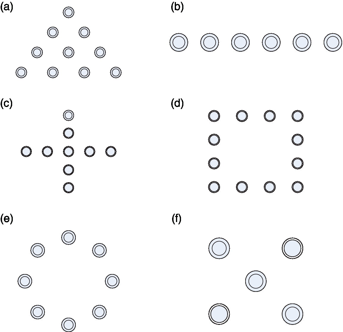
- Assume the existence of an ad hoc network as depicted in Figure 10.4 that uses table‐driven routing. Node 1 is in the communication range of all the other nodes. Additionally, node 2 is in the communication range of node 3 and node 6 and node 5 is in the communication range of node 6 and node 4. Communication range indicates the capabilities of receiving as well as transmitting in full duplex. Make an indicative table that will be stored at each node once the network has converged. Now, node 1 goes into sleep mode, starts moving towards the left for some time, and then stops and becomes active. On becoming active, it is detected that node 1 is now in the communication range only of node 5. What data will be shared among the nodes during the mobility of node 1, and what will now be the indicative routing table in each node after convergence again. Do the exercise separately for distance vector routing and link state routing.
- It has been mentioned that one of the disadvantages of proactive routing protocol is that ‘There may be certain routes over which no data packet has travelled and also by which there is a high probability that no packet will travel in the future. Still, the protocol utilizes resources to establish and regularly update such paths’. Design a network and the associated routing tables to prove that this statement is correct for certain networks.
- Consider the network given in Figure 10.8a, which runs DSR. The nodes that are in communication range of each other are connected by lines. The links are bidirectional. Now the node SN wants to transmit some data to node IN3 (the destination node in this case). How many nodes in total will receive the RREQ packet during the process of path discovery? Apart from the source and destination nodes, how many nodes will come to know about the entire path from SN to IN3? If IN 10 wants to communicate with IN 11, calculate the number of nodes receiving RREQ and the number of nodes that will gain knowledge of the route between IN 10 and IN 11. Assume the presence of no routes of any intermediate nodes in the cache at the beginning of the process.
- Consider the network given in Figure 10.8a where the lines indicate the communication range of the node. Node SN wants to transmit 2 MB of data to node IN 3. Use any ad hoc network simulation algorithm to compare the performance in terms of power consumption and bandwidth utilization to perform this activity for the following three categories of routing protocols (any specific protocol within the category may be used): distance‐vector‐based table‐driven routing, link‐state‐based table‐driven routing, and reactive routing.
- It has been said that ‘Directional routing may not work in some specific cases where the destination may not be reachable directly from the request zone owing to some obstacle before the destination or non‐availability of a one‐hop node to the destination, and thus a way around might be required’. Design a network to prove the correctness of this statement.
- Consider an ad hoc network as indicated in the figure on the following page. The lines indicate the communication range of the nodes. Geographic/location‐based routing has been implemented in the network. Node 2 wants to transmit data to node 4. Which will be the intermediate nodes involved in forwarding the packet in the case of greedy routing, DREAM, LAR, and face routing? Necessary assumptions may be made regarding the expected zone for the destination node. Will the packet reach the destination with all four routing techniques?
