54 4. TILTING VEHICLE CONTROL
min
U
r
;S
ro
W J D
N
P
kD1
U
.
k
/
r
R
ro
2
C
N
P
kD1
S
.k/
ro
Q
ro
2
s.t. W X
.
kC1
/
r
D A
rd
X
.k/
r
C B
rd
U
.k/
r
C E
rd
W
.0/
r
M
ro
X
.k/
C N
ro
U
.k/
L
ro
C S
.k/
ro
0 S
.
k
/
ro
S
ro;max
ˇ
ˇ
ˇ
U
.k/
r
ˇ
ˇ
ˇ
U
max
ˇ
ˇ
ˇ
U
.k/
r
U
.
k1
/
r
ˇ
ˇ
ˇ
U
slew;max
;
(4.20)
where S
.k/
ro
2 R
4
denotes slack variables for the roll envelope at the k th prediction step. e
disturbance is assumed to remain unchanged during the control horizon as W
.0/
. A
rd
; B
rd
; E
rd
are
the discretized matrices of A
r
; B
r
; E
r
derived from the roll model. e total cost to be minimized
is the l
2
norm of the control effort and slack variables, which are weighted by R
ro
and Q
ro
,
respectively.
e choice of the prediction horizon, as detailed in [70], should be long enough to see
the steady-state performance enhancement along with the transient degradation for an optimal
decision making. A ramp acceleration disturbance of 0:5g is applied to the system, and the
roll envelope is set as LTR
lim
D 0:5. MPC results with various prediction horizon settings are
shown in Figure 4.11. For a small prediction horizon as 0.5 s (i.e., N D 10; T D 50 ms), the
resultant tilting moment T
x
is in the wrong direction and makes LTR even worse. Results for the
optimized torque start to converge after the prediction horizon reaches 1 s. For computational
efficiency, a prediction horizon of 1 s is adopted for the control implementations.
It should also be noted that the LTR index overshoot is still noticeable as shown in Fig-
ure 4.11 with the active tilting control only. To further improve the vehicle stability, other on-
board control efforts should be incorporated, and an integrated approach is introduced in the
next section.
4.7.3 INTEGRATED STABILITY ENVELOPE
For lateral stability, a handling envelope has been proposed by researchers [81, 82]. e thresh-
olds for yaw rate .r
max
/ along with side-slip angles at rear wheels .˛
r;sat
/ are used to formulate
the envelope for lateral stability control. At each discrete control step k, this leads to
M
sh
X
.
k
/
L
sh
; (4.21)
where

4.7. HOLISTIC ENVELOPE CONTROL: MPC DESIGN EXAMPLE 55
a
y
(m/s
)φ (deg)
LTRT
x
(N.m)
6
4
2
0
1
0.5
0
-0.5
-1
0
-0.2
-0.4
-0.6
-0.8
-1
15
10
5
0
-5
0 1 2 3 4 5 0 1 2 3 4 5
0 1 2 3 4 5
× 10
4
0 1 2 3 4 5
Baseline N=10, ∆T = 50ms N=20, ∆T = 50ms N=30, ∆T = 50ms
Figure 4.11: Roll envelope control with different prediction horizons.
M
sh
D
2
6
6
4
C1 b
=
u
1 Cb
=
u
0 C1
0 1
O
42
3
7
7
5
; L
sh
D
2
6
6
4
˛
r;sat
˛
r;sat
r
max
r
max
3
7
7
5
:
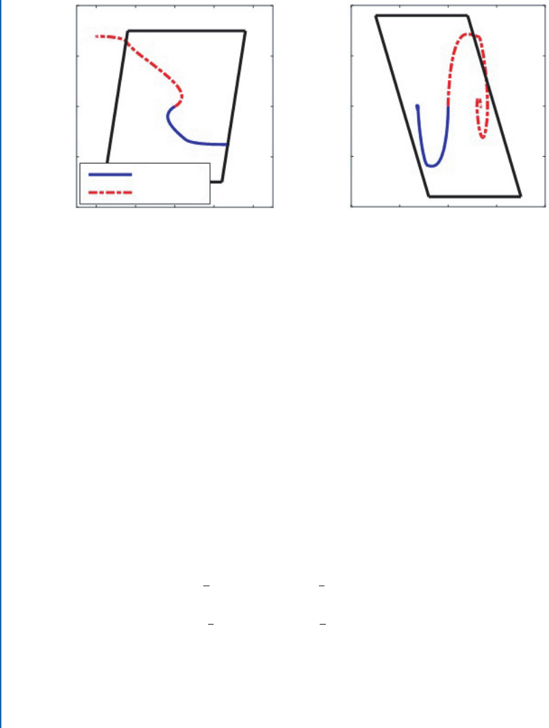
e handling envelope can be visualized in the phase plane as the boundaries shown in
Figure 4.12a. e phase plane is defined by states of lateral speed v and yaw rate r. e horizontal
boundaries stand for the yaw rate limit .r
max
/, while the sloped lines represent the constraints
for rear tire slip angle .˛
r;sat
/. For a less harsh maneuver (shown in blue) when the state trajectory
stays within the handling envelope, no control intervention is required. Active safety control will
be applied only when the system foresees the approaching of envelope violations.
By combining the handling envelope with the proposed roll envelope, an integrated en-
velope approach can be formulated, as shown in the Figure 4.12. Vehicle status is considered
safe when both lateral and roll envelope constraints are satisfied. Compared with the conven-
tional tracking approach for stability control, the proposed integrated envelope-based controller
56 4. TILTING VEHICLE CONTROL
r (rad/s)
0.4
0.2
0
-0.2
-0.4
dφ (rad/s)
0.2
0.1
0
-0.1
-0.2
-0.2 -0.1 0 0.1 0.2 -0.2 -0.1 0 0.1 0.2
Maneuver 1
Maneuver 2
v (m/s) φ (rad)
Figure 4.12: Integrated envelope approach for vehicle stability.
applies the control effort only when the predicted vehicle states are leaving the safe envelopes,
which reduces the control intervention while still maintain the desired level of stability. e
fact that lateral control efforts like active steering, torque vectoring and differential braking can
help the rollover mitigation could also be implicitly incorporated when formulating the motion
control problem in both directions as a whole.
For implementation, the integrated re-configurable model developed in Section 3.3 is
adopted. Based on that, an integrated vehicle controller with various actuator configurations
is demonstrated using the proposed envelope control scheme for both lateral and roll stability.
e controller performance, as well as robustness, is shown to be further improved with the
proposed integrated approach. e previously suggested roll envelope control Eq. (4.20) could
be extended for the integrated envelope control as
min
U;S
ro
;S
sh
W J D
1
2
N
P
kD1
U
.
k
/
R
U
2
C
1
2
N
P
kD1
r
.
k
/
r
des
R
X
2
C :::
1
2
N
P
kD1
S
.
k
/
ro
Q
ro
2
C
1
2
N
P
kD1
S
.
k
/
sh
Q
sh
2
s.t. W X
.
kC1
/
D A
d
X
.
k
/
C B
d
U
.
k
/
C E
d
W
.
0
/
M
sh
X
.k/
L
sh
C S
.
k
/
sh
S
.
k
/
sh
0
(4.22)
4.7. HOLISTIC ENVELOPE CONTROL: MPC DESIGN EXAMPLE 57
M
ro
X
.k/
C N
ro
U
.k/
L
ro
C S
.
k
/
ro
0 S
.
k
/
ro
S
ro;max
ˇ
ˇ
U
.
k
/
ˇ
ˇ
U
max
ˇ
ˇ
U
.
k
/
U
.
k1
/
ˇ
ˇ
U
slew;max
;
where A
d
, B
d
, and E
d
are discretized system matrices. S
.k/
sh
2 R
4
and S
.k/
ro
2 R
4
denotes han-
dling and roll envelope slack variables at the prediction step k. e disturbance is assumed to
remain unchanged during the control horizon as W
.0/
. e total cost to be minimized is com-
posed of control efforts, yaw rate tracking errors, and the slack variable for both lateral and roll
envelopes, which are weighted by R
U
, R
X
, Q
ro
, and Q
sh
, respectively. e desired yaw rate to
be tracked is the same as shown in Eq. (4.9).
Using the batch formulation, state trajectories in the prediction horizon, by adopting the
plant model, can be written as
N
X D S
X
X
.
0
/
C S
U 0
U
.
0
/
C S
W 0
W
.
0
/
C S
U
N
U C S
W
N
W ; (4.23)
where
N
X D
2
6
6
6
6
6
6
4
X
.
1
/
X
.
2
/
:
:
:
:
:
:
X
.
N
/
3
7
7
7
7
7
7
5
;
N
U D
2
6
6
6
6
6
6
4
U
.
1
/
U
.
2
/
:
:
:
:
:
:
U
.
N
/
3
7
7
7
7
7
7
5
;
N
W D
2
6
6
6
6
6
6
4
W
.
1
/
W
.
2
/
:
:
:
:
:
:
W
.
N
/
3
7
7
7
7
7
7
5
S
X
D
2
6
6
6
6
6
6
4
A
1
d
A
2
d
:
:
:
:
:
:
A
N
d
3
7
7
7
7
7
7
5
; S
U 0
D
2
6
6
6
6
6
6
4
B
1
d
A
d
B
d
:
:
:
:
:
:
A
N 1
d
B
d
3
7
7
7
7
7
7
5
; S
W 0
D
2
6
6
6
6
6
6
4
E
1
d
A
d
E
d
:
:
:
:
:
:
A
N 1
d
E
d
3
7
7
7
7
7
7
5
S
U
D
2
6
6
6
6
6
6
4
O O
B
d
O O
A
d
B
d
B
d
O
:
:
:
:
:
:
:
:
:
:
:
:
:
:
:
:
:
:
A
N 2
d
B
d
A
N 3
d
B
d
B
d
O
3
7
7
7
7
7
7
5
58 4. TILTING VEHICLE CONTROL
S
W
D
2
6
6
6
6
6
6
4
O O
E
d
O O
A
d
E
d
E
d
O
:
:
:
:
:
:
:
:
:
:
:
:
:
:
:
:
:
:
A
N 2
d
E
d
A
N 3
d
E
d
E
d
O
3
7
7
7
7
7
7
5
:
e envelope constraints can also be written with the batch form. For example, the roll
envelope as
M
RO
N
X C N
RO
N
U L
RO
C
N
S
ro
; (4.24)
where
M
RO
D BlockDiag
M
ro
M
ro
M
ro
N
RO
D BlockDiag
N
ro
N
ro
N
ro
L
RO
D
L
ro
L
ro
L
ro
T
N
S
RO
D
S
.
1
/
ro
S
.
2
/
ro
S
.
N
/
ro
T
:
Combining Eqs. (4.23) and (4.24) gives the design variables in the linear constraint form
A
RO
b
RO
; (4.25)
where
D
N
U
N
S
ro
N
S
sh
T
A
RO
D BlockDiag
M
RO
S
U
C N
RO
I O
b
RO
D L
RO
M
RO
S
X
X
.
0
/
C S
U 0
U
.
0
/
C S
W 0
W
.
0
/
C S
W
N
W
:
Similarly, the handling envelope can be written as
A
SH
b
SH
(4.26)
with
A
SH
D BlockDiag
M
SH
S
U
O I
b
SH
D L
SH
M
SH
S
X
X
.
0
/
C S
U 0
U
.
0
/
C S
W 0
W
.
0
/
C S
W
N
W
:
Equations (4.25) and (4.26), along with the constraints on the design variables and their
slew rate, form the linear constraint in the quadratic programming problem. e objective func-
tion in Eq. (4.22) can be rewritten by considering Eq. (4.23) as
..................Content has been hidden....................
You can't read the all page of ebook, please click here login for view all page.