Now on to our first VAE. This VAE will work with the MNIST dataset and give you a better idea about how VAEs work. In the next section, we will build the same VAE for credit card fraud detection.

Firstly, we need to import several elements, which we can do simply by running:

from keras.models import Model
from keras.layers import Input, Dense, Lambda
from keras import backend as K
from keras import metrics

Notice the two new imports, the Lambda layer and the metrics module. The metrics module provides metrics, such as the cross-entropy loss, which we will use to build our custom loss function. Meanwhile the Lambda layer allows us to use Python functions as layers, which we will use to sample from the encoding distribution. We will see just how the Lambda layer works in a bit, but first, we need to set up the rest of the neural network.

The first thing we need to do is to define a few hyperparameters. Our data has an original dimensionality of 784, which we compress into a latent vector with 32 dimensions. Our network has an intermediate layer between the input and the latent vector, which has 256 dimensions. We will train for 50 epochs with a batch size of 100:

batch_size = 100
original_dim = 784
latent_dim = 32
intermediate_dim = 256
epochs = 50

For computational reasons, it is easier to learn the log of the standard deviation rather than the standard deviation itself. To do this we create the first half of our network, in which the input, x, maps to the intermediate layer, h. From this layer, our network splits into z_mean, which expresses and z_log_var, which expresses :

x = Input(shape=(original_dim,))
h = Dense(intermediate_dim, activation='relu')(x)
z_mean = Dense(latent_dim)(h)
z_log_var = Dense(latent_dim)(h)

The Lambda layer wraps an arbitrary expression, that is, a Python function, as a Keras layer. Yet there are a few requirements in order to make this work. For backpropagation to work, the function needs to be differentiable. After all, we want to update the network weights by the gradient of the loss. Luckily, Keras comes with a number of functions in its backend module that are all differentiable, and simple Python math, such as y = x + 4, is fine as well.

Additionally, a Lambda function can only take one input argument. In the layer we want to create, the input is just the previous layer's output tensor. In this case, we want to create a layer with two inputs, and . Therefore, we will wrap both inputs into a tuple that we can then take apart.

You can see the function for sampling below:

def sampling(args):
    z_mean, z_log_var = args                                  #1
    epsilon = K.random_normal(shape=(K.shape(z_mean)[0], latent_dim), mean=0.,stddev=1.0)                     #2
    return z_mean + K.exp(z_log_var / 2) * epsilon            #3

Let's take a minute to break down the function:

All these operations are differentiable since we are using the Keras backend functions. Now we can turn this function into a layer and connect it to the previous two layers with one line:

z = Lambda(sampling)([z_mean, z_log_var])

And voilà! We've now got a custom layer that samples from a normal distribution described by two tensors. Keras can automatically backpropagate through this layer and train the weights of the layers before it.

Now that we have encoded our data, we also need to decode it as well. We are able to do this with two Dense layers:

decoder_h = Dense(intermediate_dim, activation='relu')(z)
x_decoded = Dense(original_dim, activation='sigmoid')decoder_mean(h_decoded)

Our network is now complete. This network will encode any MNIST image into a mean and a standard deviation tensor from which the decoding part then reconstructs the image. The only thing missing is the custom loss incentivizing the network to both reconstruct images and produce a normal Gaussian distribution in its encodings. Let's address that now.

To create the custom loss for our VAE, we need a custom loss function. This loss function will be based on the Kullback-Leibler (KL) divergence.

KL divergence, is one of the metrics, just like cross-entropy, that machine learning inherited from information theory. While it is used frequently, there are many struggles you can encounter when trying to understand it.

At its core, KL divergence measures how much information is lost when distribution p is approximated with distribution q.

Imagine you are working on a financial model and have collected data on the returns of a security investment. Your financial modeling tools all assume a normal distribution of returns. The following chart shows the actual distribution of returns versus an approximation using a normal distribution model. For the sake of this example, let's assume there are only discrete returns. Before we go ahead, be assured that we'll cover continuous distributions later:

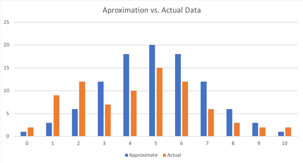
Approximation versus actual

Of course, the returns in your data are not exactly normally distributed. So, just how much information about returns would you lose if you did lose the approximation? This is exactly what the KL divergence is measuring:

Here and are the probabilities that x, in this case, the return, has some value i, say 5%. The preceding formula effectively expresses the expected difference in the logarithm of probabilities of the distributions p and q:

This expected difference of log probabilities is the same as the average information lost if you approximate distribution p with distribution q. See the following:

Given that the KL divergence is usually written out as follows:

It can also be written in its continuous form as:

For VAEs, we want the distribution of encodings to be a normal Gaussian distribution with a mean of zero and a standard deviation of one.

When p is substituted with the normal Gaussian distribution, , and the approximation q is a normal distribution with a mean of and a standard deviation of , , the KL divergence, simplifies to the following:

The partial derivatives to our mean and standard deviation vectors are, therefore as follows:

With the other being:

You can see that the derivative with respect to is zero if is zero, and the derivative with respect to is zero if is one. This loss term is added to the reconstruction loss.

The VAE loss is a combination of two losses: a reconstruction loss incentivizing the model to reconstruct its input well, and a KL divergence loss which is incentivizing the model to approximate a normal Gaussian distribution with its encodings. To create this combined loss, we have to first calculate the two loss components separately before combining them.

The reconstruction loss is the same loss that we applied for the vanilla autoencoder. Binary cross-entropy is an appropriate loss for MNIST reconstruction. Since Keras' implementation of a binary cross-entropy loss already takes the mean across the batch, an operation we only want to do later, we have to scale the loss back up, so that we can divide it by the output dimensionality:

reconstruction_loss = original_dim * metrics.binary_crossentropy(x, x_decoded)

The KL divergence loss is the simplified version of KL divergence, which we discussed earlier on in the section on KL divergence:

Expressed in Python, the KL divergence loss appears like the following code:

kl_loss = - 0.5 * K.sum(1 + z_log_var - K.square(z_mean) - K.exp(z_log_var), axis=-1)

Our final loss is then the mean of the sum of the reconstruction loss and KL divergence loss:

vae_loss = K.mean(reconstruction_loss + kl_loss)

Since we have used the Keras backend for all of the calculations, the resulting loss is a tensor that can be automatically differentiated. Now we can create our model as usual:

vae = Model(x, x_decoded)

Since we are using a custom loss, we have the loss separately, and we can't just add it in the compile statement:

vae.add_loss(vae_loss)

Now we will compile the model. Since our model already has a loss, we only have to specify the optimizer:

vae.compile(optimizer='rmsprop')

Another side effect of the custom loss is that it compares the output of the VAE with the input of the VAE, which makes sense as we want to reconstruct the input. Therefore, we do not have to specify the y values, as only specifying an input is enough:

		vae.fit(X_train_flat,
			shuffle=True,
			epochs=epochs,
			batch_size=batch_size,
			validation_data=(X_test_flat, None))

In the next section we will learn how we can use a VAE to generate data.

So, we've got our autoencoder, but how do we generate more data? Well, we take an input, say, a picture of a seven, and run it through the autoencoder multiple times. Since the autoencoder is randomly sampling from a distribution, the output will be slightly different at each run.

To showcase this, from our test data, we're going to take a seven:

one_seven = X_test_flat[0]

We then add a batch dimension and repeat the seven across the batch four times. After which we now have a batch of four, identical sevens:

one_seven = np.expand_dims(one_seven,0)
one_seven = one_seven.repeat(4,axis=0)

We can then make a prediction on that batch, in which case, we get back the reconstructed sevens:

s = vae.predict(one_seven)

The next step is broken in two parts. Firstly, we're going to reshape all the sevens back into image form:

s= s.reshape(4,28,28)

Then we are going to plot them:

fig=plt.figure(figsize=(8, 8))
columns = 2
rows = 2
for i in range(1, columns*rows +1):
    img = s[i-1]
    fig.add_subplot(rows, columns, i)
    plt.imshow(img)
plt.show()

As a result of running the code that we've just walked through, we'll then see the following screenshot showing our four sevens as our output:

A collection of sevens

As you can see, all of the images show a seven. While they look quite similar, if you look closely, you can see that there are several distinct differences. The seven on the top left has a less pronounced stroke than the seven on the bottom left. Meanwhile, the seven on the bottom right has a sight bow at the end.

What we've just witnessed is the VAE successfully creating new data. While using this data for more training is not as good as compared to using using completely new real-world data, it is still very useful. While generative models such as this one are nice on the eye we will now discuss how this technique can be used for credit card fraud detection.

To transfer the VAE from an MNIST example to a real fraud detection problem, all we have to do is change three hyperparameters: the input, the intermediate, and the latent dimensionality of the credit card VAE, which are all smaller than for the MNIST VAE. Everything else will remain the same:

original_dim = 29
latent_dim = 6
intermediate_dim = 16

The following visualization shows the resulting VAE including both the input and output shapes:

Overview of the credit card VAE

Armed with a VAE that can encode and generate credit card data, we can now tackle the task of an end-to-end fraud detection system. This can reduce bias in predictions as we can learn complicated rules directly from data.

We are using the encoding part of the autoencoder as a feature extractor as well as a method to give us more data where we need it. How exactly that works will be covered in the section on active learning, but for now, let's take a little detour and look at how VAEs work for time series.