
In this section, we will be building a simple ConvNet that can be used for classifying the MNIST characters, while at the same time, learning about the different pieces that make up modern ConvNets.
We can directly import the MNIST dataset from Keras by running the following code:
from keras.datasets import mnist
(x_train, y_train), (x_test, y_test) = mnist.load_data()
Our dataset contains 60,000 28x28-pixel images. MNIST characters are black and white, so the data shape usually does not include channels:
x_train.shape
out: (60000, 28, 28)
We will take a closer look at color channels later, but for now, let's expand our data dimensions to show that we only have a one-color channel. We can achieve this by running the following:
import numpy as np
x_train = np.expand_dims(x_train,-1)
x_test = np.expand_dims(x_test,-1)
x_train.shape
out: (60000, 28, 28, 1)
With the code being run, you can see that we now have a single color channel added.
Now we come to the meat and potatoes of ConvNets: using a convolutional layer in Keras. Conv2D is the actual convolutional layer, with one Conv2D layer housing several filters, as can be seen in the following code:
from keras.layers import Conv2D
from keras.models import Sequential

model = Sequential()

img_shape = (28,28,1)

model.add(Conv2D(filters=6,
                 kernel_size=3,
                 strides=1,
                 padding='valid',
                 input_shape=img_shape))
When creating a new Conv2D layer, we must specify the number of filters we want to use, and the size of each filter.
The size of the filter is also called kernel_size, as the individual filters are sometimes called kernels. If we only specify a single number as the kernel size, Keras will assume that our filters are squares. In this case, for example, our filter would be 3x3 pixels.
It is possible, however, to specify non-square kernel sizes by passing a tuple to the kernel_size parameter. For example, we could choose to have a 3x4-pixel filter through kernel_size = (3,4). However, this is very rare, and in the majority of cases, filters have a size of either 3x3 or 5x5. Empirically, researchers have found that this is a size that yields good results.
The strides parameter specifies the step size, also called the stride size, with which the convolutional filter slides over the image, usually referred to as the feature map. In the vast majority of cases, filters move pixel by pixel, so their stride size is set to 1. However, there are researchers that make more extensive use of larger stride sizes in order to reduce the spatial size of the feature map.
Like with kernel_size, Keras assumes that we use the same stride size horizontally and vertically if we specify only one value, and in the vast majority of cases that is correct. However, if we want to use a stride size of one horizontally, but two vertically, we can pass a tuple to the parameter as follows: strides=(1,2). As in the case of the filter size, this is rarely done.
Finally, we have to add padding to our convolutional layer. Padding adds zeros around our image. This can be done if we want to prevent our feature map from shrinking.
Let's consider a 5x5-pixel feature map and a 3x3 filter. The filter only fits on the feature map nine times, so we'll end up with a 3x3 output. This both reduces the amount of information that we can capture in the next feature map, and how much the outer pixels of the input feature map can contribute to the task. The filter never centers on them; it only goes over them once.
There are three options for padding: not using padding, known as "No" padding, "Same" padding and "Valid" padding.
Let's have a look at each of the three paddings. First, No Padding:
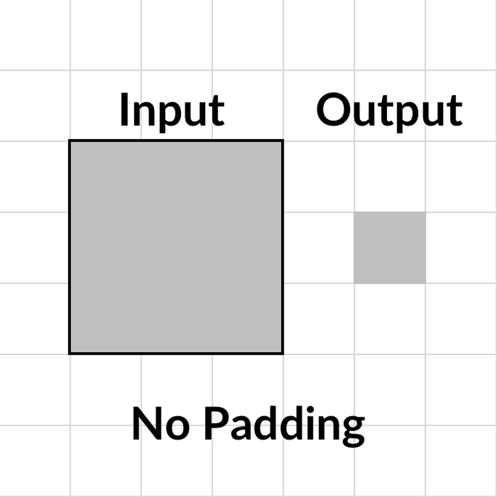
Option 1: No padding
Then we have Same Padding:

Option 2: Same padding
To ensure the output has the same size as the input, we can use same padding. Keras will then add enough zeros around the input feature map so that we can preserve the size. The default padding setting, however, is valid. This padding does not preserve the feature map size, but only makes sure that the filter and stride size actually fit on the input feature map:

Option 3: Valid padding
Keras requires us to specify the input shape. However, this is only required for the first layer. For all the following layers, Keras will infer the input shape from the previous layer's output shape.
The preceding layer takes a 28x28x1 input and slides six filters with a 2x2 filter size over it, going pixel by pixel. A more common way to specify the same layer would be by using the following code:
model.add(Conv2D(6,3,input_shape=img_shape))
The number of filters (here 6) and the filter size (here 3) are set as positional arguments, while strides and padding default to 1 and valid respectively. If this was a layer deeper in the network, we wouldn't even have to specify the input shape.
Convolutional layers only perform a linear step. The numbers that make up the image get multiplied with the filter, which is a linear operation.
So, in order to approximate complex functions, we need to introduce non-linearity with an activation function. The most common activation function for computer vision is the Rectified Linear Units, or ReLU function, which we can see here:

The ReLU activation function
The ReLU formula, which was used to produce the above chart, can be seen below:
ReLU(x) = max(x, 0)
In other words, the ReLU function returns the input if the input is positive. If it's not, then it returns zero. This very simple function has been shown to be quite useful, making gradient descent converge faster.
It is often argued that ReLU is faster because the derivative for all values above zero is just one, and it does not become very small as the derivative for some extreme values does, for example, with sigmoid or tanh.
ReLU is also less computationally expensive than both sigmoid and tanh. It does not require any computationally expensive calculations, input values below zero are just set to zero, and the rest is outputted. Unfortunately, though, ReLU activations are a bit fragile and can "die."
When the gradient is very large and moves multiple weights towards a negative direction, then the derivative of ReLU will also always be zero, so the weights never get updated again. This might mean that a neuron never fires again. However, this can be mitigated through a smaller learning rate.
Because ReLU is fast and computationally cheap, it has become the default activation function for many practitioners. To use the ReLU function in Keras, we can just name it as the desired activation function in the activation layer, by running this code:
from keras.layers import Activation
model.add(Activation('relu'))It's common practice to use a pooling layer after a number of convolutional layers. Pooling decreases the spatial size of the feature map, which in turn reduces the number of parameters needed in a neural network and thus reduces overfitting.
Below, we can see an example of Max Pooling:

Max pooling
Max pooling returns the maximum element out of a pool. This is in contrast to the example average of AveragePooling2D, which returns the average of a pool. Max pooling often delivers superior results to average pooling, so it is the standard most practitioners use.
Max pooling can be achieved by running the following:
from keras.layers import MaxPool2D

model.add(MaxPool2D(pool_size=2,
                    strides=None,
                    padding='valid'))
When using a max pooling layer in Keras, we have to specify the desired pool size. The most common value is a 2x2 pool. Just as with the Conv2D layer, we can also specify a stride size.
For pooling layers, the default stride size is None, in which case Keras sets the stride size to be the same as the pool size. In other words, pools are next to each other and don't overlap.
We can also specify padding, with valid being the default choice. However, specifying same padding for pooling layers is extremely rare since the point of a pooling layer is to reduce the spatial size of the feature map.
Our MaxPooling2D layer here takes 2x2-pixel pools next to each other with no overlap and returns the maximum element. A more common way of specifying the same layer is through the execution of the following:
model.add(MaxPool2D(2))
In this case, both strides and padding are set to their defaults, None and valid respectively. There is usually no activation after a pooling layer since the pooling layer does not perform a linear step.
You might have noticed that our feature maps are three dimensional while our desired output is a one-dimensional vector, containing the probability of each of the 10 classes. So, how do we get from 3D to 1D? Well, we Flatten our feature maps.
The Flatten operation works similar to NumPy's flatten operation. It takes in a batch of feature maps with dimensions (batch_size, height, width, channels) and returns a set of vectors with dimensions (batch_size, height * width * channels).
It performs no computation and only reshapes the matrix. There are no hyperparameters to be set for this operation, as you can see in the following code:
from keras.layers import Flatten

model.add(Flatten())
ConvNets usually consist of a feature extraction part, the convolutional layers, as well as a classification part. The classification part is made up out of the simple fully connected layers that we’ve already explored in Chapter 1, Neural Networks and Gradient-Based Optimization, and Chapter 2, Applying Machine Learning to Structured Data.
To distinguish the plain layers from all other types of layers, we refer to them as Dense layers. In a dense layer, each input neuron is connected to an output neuron. We only have to specify the number of output neurons we would like, in this case, 10.
This can be done by running the following code:
from keras.layers import Dense
model.add(Dense(10))
After the linear step of the dense layer, we can add a softmax activation for multi-class regression, just as we did in the first two chapters, by running the following code:
model.add(Activation('softmax'))Let's now put all of these elements together so we can train a ConvNet on the MNIST dataset.
First, we must specify the model, which we can do with the following code:
from keras.layers import Conv2D, Activation, MaxPool2D, Flatten, Dense
from keras.models import Sequential

img_shape = (28,28,1)

model = Sequential()

model.add(Conv2D(6,3,input_shape=img_shape))

model.add(Activation('relu'))

model.add(MaxPool2D(2))

model.add(Conv2D(12,3))

model.add(Activation('relu'))

model.add(MaxPool2D(2))

model.add(Flatten())

model.add(Dense(10))

model.add(Activation('softmax'))
In the following code, you can see the general structure of a typical ConvNet:
Conv2D
Pool

Conv2D
Pool

Flatten

Dense
The convolution and pooling layers are often used together in these blocks; you can find neural networks that repeat the Conv2D, MaxPool2D combination tens of times.
We can get an overview of our model with the following command:
model.summary()
Which will give us the following output:
Layer (type)                 Output Shape              Param #
=================================================================
conv2d_2 (Conv2D)            (None, 26, 26, 6)         60
_________________________________________________________________
activation_3 (Activation)    (None, 26, 26, 6)         0
_________________________________________________________________
max_pooling2d_2 (MaxPooling2 (None, 13, 13, 6)         0
_________________________________________________________________
conv2d_3 (Conv2D)            (None, 11, 11, 12)        660
_________________________________________________________________
activation_4 (Activation)    (None, 11, 11, 12)        0
_________________________________________________________________
max_pooling2d_3 (MaxPooling2 (None, 5, 5, 12)          0
_________________________________________________________________
flatten_2 (Flatten)          (None, 300)               0
_________________________________________________________________
dense_2 (Dense)              (None, 10)                3010
_________________________________________________________________
activation_5 (Activation)    (None, 10)                0
=================================================================
Total params: 3,730
Trainable params: 3,730
Non-trainable params: 0
_________________________________________________________________
In this summary, you can clearly see how the pooling layers reduce the size of the feature map. It's a little bit less obvious from the summary alone, but you can see how the output of the first Conv2D layer is 26x26 pixels, while the input images are 28x28 pixels.
By using valid padding, Conv2D also reduces the size of the feature map, although only by a small amount. The same happens for the second Conv2D layer, which shrinks the feature map from 13x13 pixels to 11x11 pixels.
You can also see how the first convolutional layer only has 60 parameters, while the Dense layer has 3,010, over 50 times as many parameters. Convolutional layers usually achieve surprising feats with very few parameters, which is why they are so popular. The total number of parameters in a network can often be significantly reduced by convolutional and pooling layers.
The MNIST dataset we are using comes preinstalled with Keras. When loading the data, make sure you have an internet connection if you want to use the dataset directly via Keras, as Keras has to download it first.
You can import the dataset with the following code:
from keras.datasets import mnist
(x_train, y_train), (x_test, y_test) = mnist.load_data()
As explained at the beginning of the chapter, we want to reshape the dataset so that it can have a channel dimension as well. The dataset as it comes does not have a channel dimension yet, but this is something we can do:
x_train.shape
out:
(60000, 28, 28)
So, we add a channel dimension with NumPy, with the following code:
import numpy as np

x_train = np.expand_dims(x_train,-1)

x_test = np.expand_dims(x_test,-1)
Now there is a channel dimension, as we can see here:
x_train.shape
out:
(60000, 28, 28,1)
In the previous chapters, we have used one-hot encoded targets for multiclass regression. While we have reshaped the data, the targets are still in their original form. They are a flat vector containing the numerical data representation for each handwritten figure. Remember that we have 60,000 of these in the MNIST dataset:
y_train.shape
out:
(60000,)
Transforming targets through one-hot encoding is a frequent and annoying task, so Keras allows us to just specify a loss function that converts targets to one-hot on the fly. This loss function is called sparse_categorical_crossentropy.
It's the same as the categorical cross-entropy loss used in earlier chapters, the only difference is that this uses sparse, that is, not one-hot encoded, targets.
Just as before, you still need to make sure that your network output has as many dimensions as there are classes.
We're now at a point where we can compile the model, which we can do with the following code:
model.compile(loss='sparse_categorical_crossentropy',optimizer='adam',metrics=['acc'])
As you can see, we are using an Adam optimizer. The exact workings of Adam are explained in the next section, More bells and whistles for our neural network, but for now, you can just think of it as a more sophisticated version of stochastic gradient descent.
When training, we can directly specify a validation set in Keras by running the following code:
history = model.fit(x_train,y_train,batch_size=32,epochs=5,validation_data=(x_test,y_test))
Once we have successfully run that code, we'll get the following output:
Train on 60000 samples, validate on 10000 samples
Epoch 1/10
60000/60000 [==============================] - 19s 309us/step - loss: 5.3931 - acc: 0.6464 - val_loss: 1.9519 - val_acc: 0.8542
Epoch 2/10
60000/60000 [==============================] - 18s 297us/step - loss: 0.8855 - acc: 0.9136 - val_loss: 0.1279 - val_acc: 0.9635
....
Epoch 10/10
60000/60000 [==============================] - 18s 296us/step - loss: 0.0473 - acc: 0.9854 - val_loss: 0.0663 - val_acc: 0.9814
To better see what is going on, we can plot the progress of training with the following code:
import matplotlib.pyplot as plt

fig, ax = plt.subplots(figsize=(10,6))
gen = ax.plot(history.history['val_acc'], label='Validation Accuracy')
fr = ax.plot(history.history['acc'],dashes=[5, 2], label='Training Accuracy')

legend = ax.legend(loc='lower center', shadow=True)

plt.show()
This will give us the following chart:

The visualized output of validation and training accuracy
As you can see in the preceding chart, the model achieves about 98% validation accuracy, which is pretty nice!