In previous chapters we've explained gradient descent in terms of someone trying to find the way down a mountain by just following the slope of the floor. Momentum can be explained with an analogy to physics, where a ball is rolling down the same hill. A small bump in the hill would not make the ball roll in a completely different direction. The ball already has some momentum, meaning that its movement gets influenced by its previous movement.

Instead of directly updating the model parameters with their gradient, we update them with the exponentially weighted moving average. We update our parameter with an outlier gradient, then we take the moving average, which will smoothen out outliers and capture the general direction of the gradient, as we can see in the following diagram:

How momentum smoothens gradient updates

The exponentially weighted moving average is a clever mathematical trick used to compute a moving average without having to memorize a set of previous values. The exponentially weighted average, V, of some value, , would be as follows:

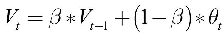
A beta value of 0.9 would mean that 90% of the mean would come from the previous moving average, , and 10% would come from the new value, .

Using momentum makes learning more robust against gradient descent pitfalls such as outlier gradients, local minima, and saddle points.

We can augment the standard stochastic gradient descent optimizer in Keras with momentum by setting a value for beta, which we do in the following code:

from keras.optimizers import SGD
momentum_optimizer = SGD(lr=0.01, momentum=0.9)

This little code snippet creates a stochastic gradient descent optimizer with a learning rate of 0.01 and a beta value of 0.9. We can use it when we compile our model, as we'll now do with this:

model.compile(optimizer=momentum_optimizer,loss='sparse_categorical_crossentropy',metrics=['acc'])

Back in 2015, Diederik P. Kingma and Jimmy Ba created the Adam (Adaptive Momentum Estimation) optimizer. This is another way to make gradient descent work more efficiently. Over the past few years, this method has shown very good results and has, therefore, become a standard choice for many practitioners. For example, we've used it with the MNIST dataset.

First, the Adam optimizer computes the exponentially weighted average of the gradients, just like a momentum optimizer does. It achieves this with the following formula:

It then also computes the exponentially weighted average of the squared gradients:

It then updates the model parameters like this:

Here is a very small number to avoid division by zero.

This division by the root of squared gradients reduces the update speed when gradients are very large. It also stabilizes learning as the learning algorithm does not get thrown off track by outliers as much.

Using Adam, we have a new hyperparameter. Instead of having just one momentum factor, , we now have two, and . The recommended values for

and are 0.9 and 0.999 respectively.

We can use Adam in Keras like this:

from keras.optimizers import adam

adam_optimizer=adam(lr=0.1,beta_1=0.9, beta_2=0.999, epsilon=1e-08)

model.compile(optimizer=adam_optimizer,loss='sparse_categorical_crossentropy',metrics=['acc'])

As you have seen earlier in this chapter, we can also compile the model just by passing the adam string as an optimizer. In this case, Keras will create an Adam optimizer for us and choose the recommended values.

Regularization is a technique used to avoid overfitting. Overfitting is when the model fits the training data too well, and as a result, it does not generalize well to either development or test data. You may see that overfitting is sometimes also referred to as "high variance," while underfitting, obtaining poor results on training, development, and test data, is referred to as "high bias."

In classical statistical learning, there is a lot of focus on the bias-variance tradeoff. The argument that is made is that a model that fits very well to the training set is likely to be overfitting and that some amount of underfitting (bias) has to be accepted in order to obtain good outcomes. In classical statistical learning, the hyperparameters that prevent overfitting also often prevent the training set fitting well.

Regularization in neural networks, as it is presented here, is largely borrowed from classical learning algorithms. Yet, modern machine learning research is starting to embrace the concept of "orthogonality," the idea that different hyperparameters influence bias and variance.

By separating those hyperparameters, the bias-variance tradeoff can be broken, and we can find models that generalize well and deliver accurate predictions. However, so far these efforts have only yielded small rewards, as low-bias and low-variance models require large amounts of training data.

L2 regularization

One popular technique to counter overfitting is L2 regularization. L2 regularization adds the sum of squared weights to the loss function. We can see an example of this in the formula below:

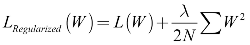
Here N is the number of training examples and is the regularization hyperparameter, which determines how much we want to regularize, with a common value being around 0.01.

Adding this regularization to the loss function means that high weights increase losses and the algorithm is incentivized to reduce the weights. Small weights, those around zero, mean that the neural network will rely less on them.

Therefore, a regularized algorithm will rely less on every single feature and every single node activation, and instead will have a more holistic view, taking into account many features and activations. This will prevent the algorithm from overfitting.

L1 regularization

L1 regularization is very similar to L2 regularization, but instead of adding the sum of squares, it adds the sum of absolute values, as we can see in this formula:

In practice, it is often a bit uncertain as to which of the two will work best, but the difference between the two is not very large.

from keras.regularizers import l2

model = Sequential()


model.add(Conv2D(6,3,input_shape=img_shape, kernel_regularizer=l2(0.01)))

model.add(Activation('relu'))

model.add(MaxPool2D(2))

model.add(Conv2D(12,3,activity_regularizer=l2(0.01)))

model.add(Activation('relu'))

model.add(MaxPool2D(2))

model.add(Flatten())

model.add(Dense(10,bias_regularizer=l2(0.01)))

model.add(Activation('softmax'))

model.compile(loss='sparse_categorical_crossentropy',optimizer = 'adam',metrics=['acc'])
              
history = model.fit(x_train,y_train,batch_size=32,epochs=10,validation_data=(x_test,y_test))

Train on 60000 samples, validate on 10000 samples
Epoch 1/10
60000/60000 [==============================] - 22s 374us/step - loss: 7707.2773 - acc: 0.6556 - val_loss: 55.7280 - val_acc: 0.7322
Epoch 2/10
60000/60000 [==============================] - 21s 344us/step - loss: 20.5613 - acc: 0.7088 - val_loss: 6.1601 - val_acc: 0.6771
....
Epoch 10/10
60000/60000 [==============================] - 20s 329us/step - loss: 0.9231 - acc: 0.8650 - val_loss: 0.8309 - val_acc: 0.8749

As the title of the 2014 paper by Srivastava et al gives away, Dropout is A Simple Way to Prevent Neural Networks from Overfitting. It achieves this by randomly removing nodes from the neural network:

Schematic of the dropout method. From Srivastava et al, "Dropout: A Simple Way to Prevent Neural Networks from Overfitting," 2014

With dropout, each node has a small probability of having its activation set to zero. This means that the learning algorithm can no longer rely heavily on single nodes, much like in L2 and L1 regularization. Dropout therefore also has a regularizing effect.

In Keras, dropout is a new type of layer. It's put after the activations you want to apply dropout to. It passes on activations, but sometimes it sets them to zero, achieving the same effect as a dropout in the cells directly. We can see this in the following code:

from keras.layers import Dropout
model = Sequential()

model.add(Conv2D(6,3,input_shape=img_shape))
model.add(Activation('relu'))
model.add(MaxPool2D(2))

model.add(Dropout(0.2))

model.add(Conv2D(12,3))
model.add(Activation('relu'))
model.add(MaxPool2D(2))

model.add(Dropout(0.2))

model.add(Flatten())

model.add(Dense(10,bias_regularizer=l2(0.01)))

model.add(Activation('softmax'))

A dropout value of 0.5 is considered a good choice if overfitting is a serious problem, while values that are over 0.5 are not very helpful, as the network would have too few values to work with. In this case, we chose a dropout value of 0.2, meaning that each cell has a 20% chance of being set to zero.

Note that dropout is used after pooling:

model.compile(loss='sparse_categorical_crossentropy',optimizer = 'adam',metrics=['acc'])
              
history = model.fit(x_train,y_train,batch_size=32,epochs=10,validation_data=(x_test,y_test))

Train on 60000 samples, validate on 10000 samples
Epoch 1/10
60000/60000 [==============================] - 22s 371us/step - loss: 5.6472 - acc: 0.6039 - val_loss: 0.2495 - val_acc: 0.9265
Epoch 2/10
60000/60000 [==============================] - 21s 356us/step - loss: 0.2920 - acc: 0.9104 - val_loss: 0.1253 - val_acc: 0.9627
....
Epoch 10/10
60000/60000 [==============================] - 21s 344us/step - loss: 0.1064 - acc: 0.9662 - val_loss: 0.0545 - val_acc: 0.9835

The low dropout value creates nice results for us, but again, the network does better on the validation set rather than the training set, a clear sign of underfitting taking place. Note that dropout is only applied at training time. When the model is used for predictions, dropout doesn't do anything.

Batchnorm, short for batch normalization, is a technique for "normalizing" input data to a layer batch-wise. Each batchnorm computes the mean and standard deviation of the data and applies a transformation so that the mean is zero and the standard deviation is one.

This makes training easier because the loss surface becomes more "round." Different means and standard deviations along different input dimensions would mean that the network would have to learn a more complicated function.

In Keras, batchnorm is a new layer as well, as you can see in the following code:

from keras.layers import BatchNormalization

model = Sequential()

model.add(Conv2D(6,3,input_shape=img_shape))
model.add(Activation('relu'))
model.add(MaxPool2D(2))

model.add(BatchNormalization())

model.add(Conv2D(12,3))
model.add(Activation('relu'))
model.add(MaxPool2D(2))

model.add(BatchNormalization())

model.add(Flatten())

model.add(Dense(10,bias_regularizer=l2(0.01)))

model.add(Activation('softmax'))
model.compile(loss='sparse_categorical_crossentropy',optimizer = 'adam',metrics=['acc'])
              
history = model.fit(x_train,y_train,batch_size=32,epochs=10,validation_data=(x_test,y_test))

Train on 60000 samples, validate on 10000 samples
Epoch 1/10
60000/60000 [==============================] - 25s 420us/step - loss: 0.2229 - acc: 0.9328 - val_loss: 0.0775 - val_acc: 0.9768
Epoch 2/10
60000/60000 [==============================] - 26s 429us/step - loss: 0.0744 - acc: 0.9766 - val_loss: 0.0668 - val_acc: 0.9795
....
Epoch 10/10
60000/60000 [==============================] - 26s 432us/step - loss: 0.0314 - acc: 0.9897 - val_loss: 0.0518 - val_acc: 0.9843

Batchnorm often accelerates training by making it easier. You can see how the accuracy rate jumps up in the first epoch here:

Training and validation accuracy of our MNIST classifier with batchnorm

Batchnorm also has a mildly regularizing effect. Extreme values are often overfitted to, and batchnorm reduces extreme values, similar to activity regularization. All this makes batchnorm an extremely popular tool in computer vision.