2

Introducing Model Serving Patterns

Serving a machine learning model is one of the most complex steps in the machine learning life cycle. In Chapter 1, we saw why serving machine learning models is challenging. Serving machine learning models involves two groups in two different domains: the ML developer develops the model and the software developer serves the model. So, we need to agree upon a common language so that we can be sure how our model will be deployed to solve a particular kind of problem. Patterns in design help software architects systematically solve complicated software engineering problems. Similarly, as we learn about design patterns in model serving, the complicated process of model serving will eventually become a piece of cake. This chapter will build on the ideas of some already used patterns for ML serving. We collect the patterns followed by developers and organize and classify those patterns. This chapter will discuss the following topics:

• Design patterns in software engineering
• Understanding the value of model serving patterns
• What are the different model serving patterns
• Examples of serving patterns

Design patterns in software engineering

In the engineering domain, a pattern indicates a common approach or strategy that can be reused. This reuse helps us to understand engineering problems and solve them easily by following the solution pattern that has been made available to us by prior engineers. That’s why, when we need to serve a website, we do not have to go back to the theory and try to reinvent the wheel every time. We know the pattern required to serve the web application, which makes our job easier. Most of the time, an engineering team writes down a runbook/docs to solve a recurring problem that appears. This helps engineers avoid debugging the problem every time, thinking of a solution, designing the solution, and applying the solution.

Design patterns are handy to nail hard software engineering problems.

The Gang of Four book on design patterns in software engineering

You might be interested to learn the software engineering design patterns from the book Design Patterns: Elements of Reusable Object-Oriented Software by Erich Gamma, Richard Helm, Ralph Helm, and John Vlissides. This book brought about such a dramatic revolution in enhancing the productivity of software development that these four authors became popularly known as the Gang of Four.

To understand how design patterns help us make better software, let’s consider a hypothetical problem scenario. We want to make software that will help to create supervised ML models based on customer requirements. It currently supports the following models:

• Linear Regression
• Logistic Regression

A naive solution for this would be the following:

class Model:
    def __init__(self, model_name, model_params):
        self.model_name = model_name
        self.model_params = model_params
class ModelTrainer:
    def __init__(self, model):
        self.model= model
    def train(self):
        if self.model.model_name == "LinearRegression":
            trained_model = linear_model.LinearRegression()https://scikit-learn.org/stable/modules/generated/sklearn.linear_model.LinearRegression.html
 trained_model.fit(self.model.model_params['X'], self.model.model_params['Y'])
            return trained_model
        elif self.model.model_name == "LogisticRegression":
            trained_model = linear_model.LogisticRegression()
    trained_model.fit(self.model.model_params['X'], self.model.model_params['Y'])
             return trained_model
# Example client calls
model = Model("LinearRegression", {"X": [[1, 1], [0, 0]], "Y": [1, 0]})
model_trainer = ModelTrainer(model)
trainer_model = model_trainer.train()

Now, let's see the problems with this call:

• When a new model needs to be added, ModelTrainer needs to be modified
• It violates the single responsibility principle, which says a class should have only a single responsibility, leading to a single reason for the modification
• If we need to add more features for each of the models, we cannot do that easily
• Maintenance becomes difficult for the following reasons: a single method contains all the responsibilities obstructing parallel development, the whole program might break because of a bad change in the single conditional block, and finding the root cause of bugs may be difficult

However, if we look at what this program is doing, it can be seen as a factory providing different trainers (for different models). Then, it becomes easier for us to visualize the problem and also use this common pattern in other similar problems.

Now, let’s modify the previous program in the following way:

class Model:
    def __init__(self, model_name, model_params):
        self.model_name = model_name
        self.model_params = model_params
class ModelTrainerFactory:
    @classmethod
    def get_trainer(cls, model):
        if model.model_name == "LinearRegression":
            return  LinearRegression Trainer(model)
        elif model.model_name == "LogisticRegression":
            return LogisticRegressionTrainer(model)
class ModelTrainer:
    def __init__(self, model):
        self.model = model
    def train(self):
        pass
class LinearRegressionTrainer(ModelTrainer):
    def train(self):
     trained_model = linear_model.LinearRegression()
        trained_model.fit(self.model.model_params['X'], self.model.model_params['Y'])
        return trained_model
# Example client calls
model= Model("LinearRegression", {"X": [[1, 1], [0, 0]], "Y": [1, 0]})
modelTrainer = ModelTrainerFactory.get_trainer(model)
trained_model = model_trainer.train()

The user now gets the desired model trainer from the factory. Whenever a new trainer is needed, we can start providing that trainer from the factory (such as starting a new product from a factory producing products without hampering other production pipelines) by adding a new trainer with a single responsibility. This program is now very easy to maintain and modify. We can use this as a template and apply it in similar problems where we need a collection of different approaches or objects. This pattern is called the factory pattern. It is a very basic but useful pattern.

Similarly, there are more than 20 different software engineering patterns that help users to approach common and repeating problems following a well-known template.

In a similar way, using patterns in ML model serving can solve recurring ML model serving problems.

In the next section, we will get a high-level overview of the patterns for serving ML models.

Understanding the value of model serving patterns

Using patterns for ML model serving make us more productive in bringing our model to clients. If we do not follow any patterns, then we may struggle to find the right tool and strategy needed to serve the model for a particular problem.

Figure 2.1 – Alice needs to perform trial and error with multiple tools to find the right one

Let’s consider the situation of Alice in Figure 2.1. Alice has a problem that involves making a data-driven decision. She needs to create a model to solve the problem and deploy the model using a serving tool. She has thousands of tools on offer. She needs to study all these solutions and find the best solution. There is another challenge in the approach of selecting the right tool. Alice is at risk of making a bad choice of tool, as she is solving an optimization problem manually and can be stuck at local maxima. This is always an impediment to productivity, as it involves extra manual effort.

Alice might often have to backtrack to find a suitable model, which creates an exponential search space for her. This situation brings a big tech debt to ML developers because the company might move forward with bad choices of tools that need to be replaced in the near future.

Let’s think about it from the point of view of hiring managers. The hiring manager now needs to solve a difficult hiring problem to find suitable talent. They will have difficulties and challenges finding skilled developers who can come up with a solution within a reasonable amount of time. It might be more intuitive to think mathematically about why finding a skilled developer may be hard. Let’s say that company A usually faces P kind of problems, each of which needs a different model serving approach. There are N different tools available to serve the model.

So, for each problem, a developer needs to try N tools before finding a satisfactory solution. Therefore, for P problems, there will be PN different choices for the developer, and in the worst-case scenario, the developer might have to try all these choices to find the best option. Through experience and observations, developers will be able to create a shortlist of the best tools to avoid trying all the choices, and their knowledge of model serving patterns will help the developer to easily make that shortlist. This creates a big bottleneck in productivity. The learning curve to getting skilled in these tools is high. The developer needs to learn the pros and cons of each tool for a particular problem. Therefore, getting a sufficiently skilled developer who can serve the model efficiently becomes hard.

Figure 2.2 – Bob takes the problem pattern and matches it with a few solution patterns

Conversely, let’s consider Bob in Figure 2.2. As the category of ML problems can be served using only a few recurring patterns, he can quickly map a problem to the serving strategy or pattern needed.

If a problem is encountered, he can quickly map the problem to a suitable serving pattern. Serving becomes a very easy step in the ML life cycle for Bob. Let’s revisit the same math problem as before. Now, Bob only has to apply a single pattern for a problem. So, for P problems, he only needs to go deeper into a few patterns. This makes the learning curve easier for a new developer and brings benefits to both the developers and the AI industry.

From this hypothetical scenario, we get the idea that we should follow pattern-oriented approaches in model serving instead of following tool-oriented approaches.

Here are some of the reasons why we need to know model serving patterns:

• Resilient serving: The served models should be fault-tolerant and should have mechanisms to recover from faults automatically. However, if we blindly try different approaches and tools without looking at the patterns, we might insert many loopholes, creating issues such as scalability problems and model versioning issues. We might also have difficulty in updating the model without causing problems if patterns are not followed, hampering resilient serving.
• Using well-vetted solutions: Using model serving patterns, we can reuse existing solutions to reduce production time. As these approaches are practiced by the developers, these approaches have become trusted and are supported by strong communities. After serving, we can be more confident and also get immediate support if needed.
• Steep learning curve: It is obvious that training engineers on model serving becomes much easier when we have patterns ready to hand. The engineers are taught the patterns, and they can follow these patterns to serve a new model without going through an array of tools to select the best one. So, patterns help make the learning curve to get skilled in model serving much smoother.
• Development of sophisticated serving techniques: Patterns can help you to develop abstract tools that are specialized for particular patterns. By abstract tools, I mean that the tool hides all the implementation details and provides an easier UI interface for users. For example, let’s consider the online serving pattern. We can develop abstract tools to serve in real time by simply connecting our stream of data to the tool that already abstracts the background processes and complex logic needed for online learning, as shown in Figure 2.3.

Figure 2.3 – This pattern can help to develop abstract pattern-oriented serving tools

From Figure 2.3, we can see that the user is serving models using a tool based on an online model serving pattern. The user does not have to do a lot of complicated tasks such as data cleaning, feature selection, model selection, training, and choosing serving techniques. The user only plugs in the input data to the hypothetical tool and gets the predictions from the APIs exposed to the tool. When we understand the serving patterns for different problem types, developing these tools will be easier.

As Bob is gaining all these advantages from using patterns, he has happy users and a more robust model serving pipeline. On the other hand, as Alice is not following any pattern, she is at high risk of the model experiencing downtime, a sudden drop in performance making clients unhappy, and also dealing with the flaky nature of model inference.

ML serving patterns

There are patterns that are specific to serving ML models. In this section, we will discuss the patterns for ML model serving. We will see the categories of patterns and describe each of the categories separately.

Model serving patterns can be classified into the following two categories at a high level:

• Serving philosophies: This group of patterns mainly concerns the principles and best practices you need to be aware of when serving a model – for example, whether the serving should be stateful or stateless, or whether we should evaluate the performance of the model continuously or intermittently
• Serving approaches: This kind of pattern gives a clear picture of different serving approaches – for example, how the model will be served in cases of the presence of a large quantity of distributed data, how the model will be served if we need the immediate impact of the most recent data, or how we will serve on edge devices

We will look at these two categories in more detail in the following subsections. We will describe the two categories and see the patterns under each of these categories.

Serving philosophy patterns

In this section, we will learn about the patterns in model serving that describe the state-of-the-art principles in model serving. We place these patterns under the class of patterns for serving philosophies.

These patterns give us ideas about the best practices that we should follow whenever we want to serve models. These patterns, instead of suggesting a particular deployment strategy, provide principles we should follow in all the serving strategies. From these kinds of patterns, we learn to make model serving resilient, available, and consistent, meaning that the responses are the same given the same input. For serving web applications, there are already agreed-upon principles and protocols – for example, communication to a server happens through REST APIs. Similarly, in this section, we will learn some standard principles for ML model serving.

Based on serving philosophies, we can classify serving patterns into three categories, as introduced in the book Machine Learning Design Patterns by Michael Munn, Sara Robinson, and Valliappa Lakshmanan:

• Stateless serving
• Continuous model evaluation
• Keyed prediction

We want to avoid stateful serving. That is an anti-pattern and should not be classified as a pattern for serving.

Stateless serving

In web serving, the server does not store any state information, meaning any client data needed to serve the calls for that particular client (we will go into more detail on states in Chapter 3, Stateless Model Serving). The user needs to transfer all the necessary states if they want to use the web service using a REST API. Anyone who needs to access a web service needs to provide the state information needed, and the web service will store that state information in the placeholders to return the desired response after processing. This ensures the scalability of web APIs, as they can be deployed to any server on an on-demand basis.

REST APIs

Representational State Transfer (REST) is a set of architectural constraints for designing APIs. For further reading on REST APIs, please read the original thesis by Roy Thomas Fielding (https://www.ics.uci.edu/~fielding/pubs/dissertation/top.htm) that introduced REST, and we can also use the following link to learn about it at a high level: https://www.redhat.com/en/topics/api/what-is-a-rest-api.

Whenever we want to make our application stateful – or the business logic demands the application needs to be stateful – then we need to be very careful. In web serving, there is a lot of talk about stateless and stateful serving. Both might be used depending on the requirements of the application. In web applications, states in stateful serving mainly refer to the states or status information in the previous calls. However, in model serving, most of the states will come from the states of the model. If the model stores state during serving, then the model might give different results for the same input at different times.

Let’s imagine there is a website to check the time at a given location. Whenever a particular user wants to use the application, the user needs to pass the location information along with the API call. Let’s also imagine for a moment that the server stores this state information (location). A user from Los Angeles has made a request to the web service to get the current time. The web service got the location information, stored it within its global state, and returned the information. At the same time, if another user from Sydney makes a request to get the time, they might get the wrong time, as the state in the server points to Los Angeles. Therefore, the application becomes buggy and also not scalable.

We can see graphically in Figure 2.4 that a stateful application that is storing states within the server can cause inconsistent results. A call, Call 1, to the server is made to the server, and before it is processed, another call, Call 2, is made. Call 2 will now have access to the states from Call 1 that the server has stored in its different placeholders or variables. Therefore, there might be inconsistent results in both Response 1 and Response 2.

Figure 2.4 – The stateful server stores states

On the contrary, a stateless server requires the client to pass the necessary states. The server is blind to the states of any call and does not store anything related to a call. Each call is served individually and independently. Each of the calls is independent of other calls and does not show any side effect that would result from the mingling of states between the calls.

As shown in Figure 2.5, the server does not store any states, and the parallel calls, Call 1 and Call 2, are independent and do not have access to the states of one another.

Figure 2.5 – Stateless serving requires the client to pass states

You got the idea of how stateful serving can be problematic. There are many side effects to allowing states within served applications. Some common problems include the following:

• Scaling the application is difficult: Whenever we need to deploy the application to a different server, we also need to save the states to the new server. This makes it difficult to scale, and the user might get different results at different times.
• The results are not consistent: As the stateful server stores previous states, a new call might use state information from the previous call, giving totally inconsistent results.
• Security threat: State information from previous users might be leaked to the new user, which brings the possibility of serious privacy and security threats.

In ML, we have different states that are used during training the model. To export the model for serving using the stateless serving principle, we need to avoid exporting these parameters. Due to the probabilistic nature of the model, sometimes we use different random states during training. While serving the application, we need a mechanism to get rid of this. Otherwise, this will create a bad user experience, as the user will keep getting different results for the same call at different times. Clients might become intolerant of the probabilistic nature of the response from the models, as they are more interested in getting consistent results.

As an example, to understand the problem that stateful model serving might create, let’s say a developer has demoed an application to a team manager, and they have seen the result, R1. Now, the demo is given to a program manager, and the result is R2. This will create distrust and a lack of confidence among the production team as well. Also, if the users start using it and they keep getting different results, R1, R2, and R3, at different times, then it will create a bad customer experience and a high churn rate.

Therefore, we need to use a stateless serving pattern as much as we can. This makes client code and responsibility a little complicated because the client side needs to take a lot of responsibility in extracting the states from the model. However, the hope is that, in the future, more tools will come to remove this client burden.

Sometimes, making stateless serving might be really difficult. For example, let’s consider a chatbot application. It needs to store the previous state to make the answers and responses more reasonable.

Continuous model evaluation

One of the key differences between model serving and web serving is that ML models evolve based on data. An ML model will become useless quickly as more and more new example cases appear that aren't taken into account by the model.

For example, let’s say that there is a model to detect the house price of a fast-growing city. The model will become stale very soon. Let’s say the hypothetical price of a house today is $300,000. After 2 months, the price may become $500,000. So, the model that is developed today cannot be used to make predictions after 2 months. But in a web application, the functionalities of the existing feature do not usually change and the requirements are deployed incrementally step by step. Usually, the deployed requirements do not change significantlly after the User Acceptance Testing (UAT) is completed.

For example, a feature for user registration might remain exactly the same for years in a web application. However, ML models might need frequent upgrades, as data is growing every day. If we continue to use an old model, then it might suffer from the following problems:

• Use of stale data: The model was trained using some data that got stale after a certain period. For example, we can take the use case of house price prediction. Suppose the model was trained with a feature (three bedrooms and two bathrooms) and a target value of $300,000. But the data could become stale after 2 months after which there is a new target value of $500,000 for the same feature. This problem is common in ML. Formally, this problem is known as concept drift and data drift. To learn more about this, please follow this link: https://analyticsindiamag.com/concept-drift-vs-data-drift-in-machine-learning/. So, if the model is not updated, the model might be totally useless after a certain period of time.
• Underfitting: As new features come in with time, a trained model will behave like an underfitted model in the midst of a new large volume of data. Underfitting is a well-known problem that arises if the model is too simple or an insufficient amount of data is used during training. With the new volume of data, an old model will show the impact of underfitting even though it was a very robust model before.

So, we should follow the philosophy of evaluating the model continuously and setting a threshold point at which the model needs to be upgraded.

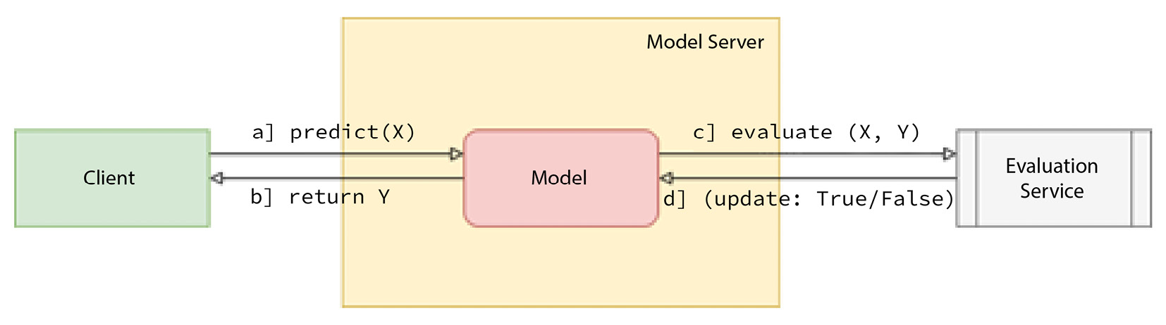
Figure 2.6 – A high-level overview of the continuous evaluation of an ML model

In Figure 2.6, we see a high-level overview of serving following the continuous evaluation pattern. Here, we serve the model, and its prediction performance is evaluated using an evaluation service. The evaluation service determines whether we should retrain the model or not based on the performance of the model.

In summary, we need to evaluate the model event after deployment and retrain when it no longer performs well. We can’t stay silent after the model is deployed, as the model performance will decay over time.

Keyed prediction model serving

Consider a case where we have a model being served for predicting the house price in a city in the USA. We pass a single input to the model (3 bedrooms and 2 bathrooms), and we get the output of $300,000. This looks very simple for a single-in and single-out case.

However, let’s say we send a batch request to the server and the features are provided as an array. Let’s assume the input feature array is [(3, 2), (2, 2), (4, 2)]. Now, we get an output of [$300k, $250k, $400k]. Now, if you are asked what kind of house has a price of $250,000, you will answer with the house whose features are (2, 2), meaning it has two bedrooms and two bathrooms. This seems a very fair claim. However, there is a problem here. The answer is assuming the requests are processed sequentially and the response array is filled up sequentially, according to the sequence input features are passed in. Let’s pause for a second and think: does this system scale well? If the number of instances in the batch request increases, the time to get a response will keep increasing linearly.

We should rather take advantage of the distributed nature of the servers and parallelize the computation. So, let’s say that for our request, the (3, 2) feature has gone to server S1, the (2, 2) feature has gone to server S2, and the (4, 2) feature has gone to server S3. The prediction by server S3 is completed first, then by server S2, and finally, server S1 completes the prediction for (3, 2). So, the response array is now jumbled, and we get [$400, $250k, $300k].

Now, if we are asked what kind of house has a price of $400,000 and we answer houses with three bedrooms and two bathrooms, our answer will be wrong.

A keyed prediction model serving pattern now comes into the picture to solve this problem and enable scalability in the serving of an ML model. The client supplies a key along with the features so that the responses can be identified using the key later on. The key can be any value that is distinct and can be used to map to the input instances easily. For example, the key can be as simple as the row number or index of the array element in the input data. The purpose of the key is to be able to match the response against the input instance.

Let’s revisit the preceding problem by passing keys now. The request now contains the following instances: [(k1, 3, 2), (k2, 2, 2), (k3, 4, 2)]. The response now will be [(k3, $400), (k2, $250k), (k1, $300k)]. Therefore, we can easily identify which response belongs to which feature set. Therefore, our problem of leveraging distributed serving is now resolved.

Patterns of serving approaches

In this section, we will discuss the serving patterns that give a clear picture of different serving approaches. These patterns describe which strategy should be followed to serve a particular type of model. These patterns are placed under the classification of patterns of serving approaches.

Serving approaches involve well-vetted strategies to serve an ML model to production – for example, where the model will be served in an online fashion so that the impact of fresh data is immediately visible in the trained model, or in batch mode where the model updates with new training data after some interval. Patterns based on serving approaches categorize different serving strategies.

Some of the main differences between serving philosophy patterns and serving approach patterns include the following:

• A serving philosophy specifies the steps or techniques of serving as fundamental practices. For example, “during serving, you should log your history” is a serving philosophy. The serving will still work even if we do not do it – there will be no impact on the serving, but we will be missing a philosophically ideal practice.
• A serving philosophy proposes a set of best practices, but a serving strategy covers a set of steps.
• A serving philosophy will not be visible directly, but a serving approach will be – for example, if we serve using a pipeline pattern, we will be able to see the pipeline. However, if we follow a good philosophy of stateless serving, that won’t be visible externally.

Based on serving approaches, we can see the following patterns in model serving:

• Batch model serving
• Online learning model serving
• Two-phase model serving
• Pipeline pattern
• Ensemble pattern
• Business logic patter

Batch model serving

Predictions from an ML model are not often possible instantly in a synchronous fashion. Whenever we need a prediction for a single feature set or a small array of feature sets, we might get the response instantly. However, when we need prediction for a large number of instances, we often need to do it asynchronously in a batch manner because of the following reasons:

• The number of instances that need prediction is very high
• The background dataset that needs to be used for training the model is high and the model needs retraining before serving each batch prediction request

For example, let’s consider creating monthly sales predictions for different items at different locations of a retail store. For that, we need predictions for thousands of features (locations and items) every month so that the demand planners can make appropriate monthly estimates of sales. For this, the following steps need to take place:

1. The model needs to be updated with large-scale sales data for the last month.
2. The model needs to be redeployed after training with the new data.
3. The model needs to make sales predictions for every feature (location and item).

For example, let’s consider the following hypothetical sample prediction of a retail store, X, in Miami, Florida:

• (Miami – apple) -> 20,000 units
• (Miami – swimming goggles) -> 5,000 units

Additionally, for the location in Miami alone, we might need predictions for thousands of items. Considering all the different locations besides Miami, the number of instances needing prediction will be very large, and the prediction needs to happen only after the model is retrained with a new volume of data.

The batch serving pattern deals with this kind of problem, where the model serving solves these batch prediction problems and makes predictions asynchronously in situations when response latency is a big concern.

Online model serving

In online prediction, the model needs to make a prediction immediately after the request is made. Usually, the model makes predictions for a single instance or a small number of instances that can be provided via the HTTP payload limit. In this kind of model, we aim for less latency to provide a better customer experience.

In online models, the model is updated with new features each time a user makes a request using continual learning/online models.

The major advantage of online model serving is that the model stays updated with new data and we can avoid the challenge of retraining.

However, there are some problems that need to be kept in mind while serving the model using the online model serving pattern. Some of these include the following:

• Model bias: The model can be converted to a biased model, as the prediction request is available only for a single target class. For example, let’s consider we have an online model for deciding on credit applications. If the prediction request comes from only positive cases, then the model might be biased towards predicting positive.
• Adversarial attacks: Online models can be susceptible to adversarial attacks. We might need an adversarial detection mechanism before passing the input to the model. Adversarial attacks are also an issue in offline models, but one additional vulnerability of online models is that the attacker can hack the live data ingestion pipeline in online models to provide malicious data.
• If the models are served through multiple servers, then the models will diverge from one another after a short period of time. For example, the model in one server might get a request and get updated, whereas the models in other servers might still stay the same.

Two-phase prediction model serving

In this pattern, two models are served; usually, one model stays on the cloud and the other on the edge devices, but there are other possible differences, including model size or other properties about which we may care. The model on the cloud is often complex and heavy. When handheld edge devices are clients of these models, we have to be aware of the problem that the edge device might be offline or in a weak connection zone. So, we need a lightweight model to be deployed on the edge device to serve the functional requirements within a Service Level Agreement (SLA).

Pipeline model serving

In serving ML, often a complex task is broken down into multiple steps, and each step focuses on a particular ML task. We can structure these steps in the form of a pipeline.

For example, let’s imagine we have a computer vision model where we identify different objects from an image or video and provide captions to the objects. The different steps involved in this whole process might be as follows:

1. Preprocess the image.
2. Use an ML model to detect the bounding boxes.
3. Use an ML model to identify the key points.
4. Another Natural Language Processing (NLP) model provides captions based on the key points.

All these separate steps can reside in a separate block in a pipeline. This will give us some flexibility in restarting the pipeline from a failed step whenever needed and debugging the process in a more granular way.

Ensemble model serving

An ensemble pattern comes becomes useful when we need to use predictions from multiple models. This blog gives overviews on ensemble and business logic patterns: https://www.anyscale.com/blog/considerations-for-deploying-machine-learning-models-in-production. Some use cases of using ensemble model serving include the following:

• Updating the model: After updating the model, we can immediately discard the old model. However, this has some risks. What if the new model does not perform as well as the old model on unseen live data? To avoid this situation, we keep both the old and new models served in an ensemble fashion and then we take the predictions from both models. We keep returning the predictions from the old model during the evaluation period and use an evaluator to evaluate the performance of the new model. Once we are satisfied with the performance of the new model, we can remove the old model.
• Aggregating the predictions from multiple models: Often, we need to get predictions from multiple models and aggregate the output either by averaging (for regression) or voting (for classification). This helps us to make more confident predictions.
• Model selection: We might have multiple models for different tasks. For example, in the category of vehicle detection, one model may be specialized in detecting cars and another model may be specialized in detecting trucks. So, based on the input feature set, we have to select the right model. Also, the items needing prediction may be from totally different groups. For example, let’s say a big retail store has separate models for predicting the price of different groups of items because their feature sets are totally different. The feature set of a grocery item is different from the feature set of a children’s toy. So, the company might be interested in having separate models trained for these different types of predictions and the models can remain ensembled, and based on the input feature, we can dynamically select which model to use for prediction.

The preceding scenarios require an ensemble serving pattern, as more than one model is ensembled or stacked together. The serving needs to accommodate this logic to support these problem scenarios.

Business logic pattern model serving

Model serving often requires a lot of business logic to be performed before inference can take place. Any logic that takes place other than inference falls into business logic. Some common business logic includes the following:

• Checking user credentials
• Loading the model from some storage such as S3
• Validating input data
• Preprocessing input data
• Loading precomputed features

These business logic functions require expensive I/O operations. Often, the inference server where the model is served is kept separate from the server where business logic is deployed. Only when the business logic is successful can a user invoke the inference API. For example, confidential military-purpose ML models might not be accessible to any users except those authorized. We need to add business logic to check that authorization. We might have to check for sensitive and malicious data in the input and need business logic to do this. We might have to add business logic to prevent Distributed Denial of Service (DDoS) attacks.

Summary

In this chapter, we have learned about the patterns in model serving. We have learned that patterns in model serving can be seen from two angles at a high level: serving patterns based on serving philosophies and serving patterns based on serving strategies.

Serving patterns based on serving philosophies involve the best practices in serving models. These patterns help us ensure resilient model serving by ensuring fault-tolerant, scalable processes in model serving.

Serving patterns based on serving strategies involve recurring approaches used for serving models for different business use cases – for example, a batch serving strategy if the predictions are not necessary immediately and online serving if the predictions are needed immediately.

We also discussed a high-level overview of each of the patterns. We saw that the serving principles such as stateless serving, continued model evaluation, and keyed prediction can help the uninterrupted and resilient serving of the model.

The serving strategy patterns such as batch serving, online serving, two-phase model serving, pipeline patterns, ensemble patterns, and business logic patterns can help us to serve models for different business use cases.

These kinds of patterns can help reduce tech debt in model serving and inspire the future development of pattern-oriented model serving tools.

Further reading

In this section, you can find some further reading that can help you to do further study of the concepts we discussed in this chapter:

• Machine Learning Design Patterns by Michael Munn, Sara Robinson, and Valliappa Lakshmanan
• REST APIs: https://restfulapi.net/