8

Two-Phase Model Serving

In this chapter, we will discuss the two-phase prediction pattern. In the two-phase prediction pattern, we deploy two different models. The bigger and more complex model is deployed on the server. In most cases, the users of this model are edge devices where the network may fluctuate. So, in the case of bad network access, an edge device can use a lightweight model to get predictions for basic use cases. For broader and more accurate predictions, the devices can get the prediction by calling APIs to the model deployed to the server. We will discuss the serving of models in this scenario of edge devices that exist in unstable networking conditions.

We will cover the following topics in this chapter:

• Introducing two-phase model serving
• Exploring two-phase model serving techniques
• Use cases of two-phase model serving

Technical requirements

In this chapter, we will use the TensorFlow library in addition to the libraries we have used before. We will be using the TensorFlow Lite converter to convert the large model to a smaller model. You should have Postman or another REST API client installed in order to send API calls and see the responses. All the code for this chapter is provided at https://github.com/PacktPublishing/Machine-Learning-Model-Serving-Patterns-and-Best-Practices/tree/main/Chapter%208.

If you get ModuleNotFoundError while trying to import any library, then you should install that module using pip3 install <module_name>. To find the exact versions of different modules, please look at the requirements.txt file in the repository.

Introducing two-phase model serving

In this section, we will discuss the basic concepts related to the two-phase model serving pattern.

The two-phase model serving pattern deploys two models for prediction. One large model is deployed on the distributed server, and one small model is deployed on the edge device. The large model is usually beyond the memory limit of the edge device and thus can’t be deployed there. The smaller model deployed on the edge device is called the phase one model. The large model deployed on the cloud is known as the phase two model. This model is large and updated frequently to provide the most accurate predictions.

Two-phase model serving is very important when edge devices are involved in the overall system, and the predictions on these edge devices are essential, irrespective of the network conditions.

The phase one model is used for making predictions for two main reasons:

• To provide predictions if the device is offline. These predictions are not as accurate as the big model’s predictions. However, these predictions are OK for getting an overview of the situation, such as getting the weather forecast or a route planner while offline. A diagram of two-phase serving in this scenario is given in Figure 8.1:

Figure 8.1 – Two-phase model serving scenario addressing offline state predictions

• To avoid calling APIs to the large model for unnecessary observations, we can keep calling the prediction API to the large model. However, this can be expensive. So, we call the phase one model to make a preliminary decision on whether we should call the API or not. For example, let’s say we have a goal to predict the categories of tigers in a forest. We can have a phase one model in an edge device that will make a binary decision of whether the observed animal is a tiger or not. If the observation is yes, then we can send the features to the phase two model to determine the classification of the tiger’s type. An example overview diagram of this serving is shown in Figure 8.2:

Figure 8.2 – High-level diagram of two-phase serving where the phase two model is called based on the prediction of the phase one model

In this section, we have seen an overview of two-phase model serving. In the next section, we will discuss the techniques required in two-phase model serving.

Exploring two-phase model serving techniques

Two-phase model serving can be one of the following three types, depending on the strength of the models:

• Quantized phase one model
• Separately trained phase one model with reduced features
• Separately trained different phase one and phase two models

Quantized phase one model

With this type, we first develop the phase two model to be deployed on the server. Then, we carry out integer quantization of the phase two model to form the phase one model. Integer quantization is an optimization technique that converts floating point numbers to 8-bit integer numbers. This way, the size of the model can decrease by a certain degree.

For example, if we convert 64-bit floating point numbers to 8-bit integers, we can get up to an 8-times reduction (64/8 = 8). A basic example of reducing the size of a floating point NumPy array to a uint8 NumPy array is shown in the following code block:

import numpy as np
import sys
X = [
    [1.5, 6.5, 7.5, 8.5],
    [1.5, 6.5, 7.5, 8.5],
    [1.5, 6.5, 7.5, 8.5],
    [1.5, 6.5, 7.5, 8.5]
]
A = np.array(X, dtype='float64')
B = A.astype(np.uint8)
print(A)
print(sys.getsizeof(A))
print(B)
print(sys.getsizeof(B))

In this code snippet, we take a NumPy array of floating point numbers and then convert the type of the array to uint8. We compute the size of the arrays in bytes before and after the conversion using sys.getsize. We get the following output from the code snippet:

[[1.5 6.5 7.5 8.5]
[1.5 6.5 7.5 8.5]
[1.5 6.5 7.5 8.5]
[1.5 6.5 7.5 8.5]]
240
[[1 6 7 8]
[1 6 7 8]
[1 6 7 8]
[1 6 7 8]]
128

So, we notice the floating-point numbers are all converted to integers, and the size of the array is reduced from 240 bytes to 128 bytes after the conversion.

The weights and biases in a deep neural network are represented by 32-bit floating point numbers. Therefore, after 8-bit integer quantization, we can reduce the size of the model by 32/8 = 4 times.

To demonstrate the reduction in the size of the model after quantization, we will use the example at https://www.tensorflow.org/lite/performance/post_training_integer_quant.

We will train a model for the MNIST dataset and then save it. We will compute the size of the saved model. Then we will do full integer quantization and save the quantized model, then finally, we will compute the size of the quantized model.

Training and saving an MNIST model

In this section, we will train a basic deep-learning model for recognizing the MNIST digits. We will follow the following steps to train and save the trained model:

1. First of all, we download the MNIST data using the following code snippet:

   mnist = tf.keras.datasets.mnist

   (train_images, train_labels), (test_images, test_labels) = mnist.load_data()
2. Then, we normalize the data using the following code snippet:

   train_images = train_images.astype(np.float32) / 255.0

   test_images = test_images.astype(np.float32) / 255.0
3. Then we define the sequential model structure as follows:

   model = tf.keras.Sequential([

     tf.keras.layers.InputLayer(input_shape=(28, 28)),

     tf.keras.layers.Reshape(target_shape=(28, 28, 1)),

     tf.keras.layers.Conv2D(filters=12, kernel_size=(3, 3), activation='relu'),

     tf.keras.layers.MaxPooling2D(pool_size=(2, 2)),

     tf.keras.layers.Flatten(),

     tf.keras.layers.Dense(10)

   ])

We can see that the model has six layers.

4. Then we compile and train the model using the following code snippet:

   model.compile(optimizer='adam',

                 loss=tf.keras.losses.SparseCategoricalCrossentropy(

                     from_logits=True),

                 metrics=['accuracy'])

   model.fit(

     train_images,

     train_labels,

     epochs=5,

     validation_data=(test_images, test_labels)

   )

Notice the final accuracy of the model in the terminal as the model finishes training:

Epoch 5/5
1875/1875 [==============================] - 15s 8ms/step - loss: 0.0602 - accuracy: 0.9826 - val_loss: 0.0633 - val_accuracy: 0.9798

We see that the model has ~98% accuracy in detecting the digits from the MNIST dataset.

5. We save the model using model.save("mnist"). We will see that the model is saved to the mnist directory, and the directory structure is shown in Figure 8.3:

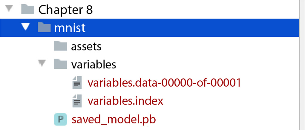
Figure 8.3 – Directory structure of the saved neural network to detect MNIST digits

Full integer quantization of the model and saving the converted model

Now we will do the full integer quantization of the model. We will use Tensorflow Lite converter tf.lite.TFLiteConverter.from_keras_model to perform the full integer quantization of the model.

1. First, we create a converter using the following code snippet:

   converter = tf.lite.TFLiteConverter.from_keras_model(model)

This code creates a converter using tf.lite.TFLiteConverter.from_keras_model and it takes the model that we created earlier as a parameter.

2. We are going to do full integer quantization, so we need to specify the representative dataset for the converter. We create the representative dataset from the training data in the following way and assign that representative data to the representative_dataset property of the converter:

   def representative_data_gen():

     for input_value in tf.data.Dataset.from_tensor_slices(train_images).batch(1).take(100):

       yield [input_value]

   converter.representative_dataset = representative_data_gen
3. Now we set the optimization strategy and the types of conversion as follows:

   converter.optimizations = [tf.lite.Optimize.DEFAULT]

   converter.target_spec.supported_ops = [tf.lite.OpsSet.TFLITE_BUILTINS_INT8]

   converter.inference_input_type = tf.uint8

   converter.inference_output_type = tf.uint8

We have set the optimizations to the default tf.lite optimization strategy. We have also set the inference_input_type and inference_output_type values to tf.uint8.

4. We can now convert the model to the quantized model using the following command:

   tflite_model_quant = converter.convert()

We have now converted the model and stored the quantized and reduced model to the tflite_model_quant variable.

5. We can save the quantized model to our local directory using the following code snippet:

   tflite_models_dir = pathlib.Path("quantized_model/")

   tflite_model_quant_file = tflite_models_dir/"mnist_model_quant.tflite"

   tflite_model_quant_file.write_bytes(tflite_model_quant)

We have saved the model in the quantized_model directory. If the directory does not exist, you might need to create the directory in your project folder before running this code.

Figure 8.4 – Directory structure of the saved quantized model

The model is saved with the name mnist_model_quant.tflite. The directory structure of the saved model is shown in Figure 8.4.

Comparing the size and accuracy of the models

We now have two models. One model is the large model where the weights and biases are in the float32 form. This is used as the phase two model, which will be deployed on the server. In our example, we saved the model with the name saved_model.pb. The other model is the quantized model, where the weights and biases use the uint8 types. Let’s compare the sizes of the two models:

1. Let’s create a separate program with the following code snippet:

   import os

   size = os.stat('mnist/saved_model.pb').st_size

   print("Size of phase two model ", size)

   size2 = os.stat('quantized_model/mnist_model_quant.tflite').st_size

   print("Size of phase one model ", size2)

   reduction = round(size/size2, 2)

   print("Reduction of size is ", reduction, "times")

From this code snippet, we get the following output:

Size of phase two model  97916
Size of phase one model  24576
Reduction of size is  3.98 times

The quantized model is almost four times smaller. However, the phase two model has some other artifacts, such as variables and assets, along with the model, as shown in Figure 8.3. We can check the sizes of these variables by going inside the directory. The size of these variables is shown in Figure 8.5. We can see that the variables are nearly three times the size of the model. Therefore, the actual reduction after quantization is much more than we got by comparing the model file sizes.

Figure 8.5 – The sizes of the items in the variables folder for the phase two model

The MNIST model is simple, so the sizes are small. For complex models, the sizes can be very big.

2. To evaluate and get predictions from the model, we first need to create an interpreter and get predictions from the interpreter. We compute the predictions from the quantized model with the following code for each of the test images:

   test_image_indices = range(test_images.shape[0])

   interpreter = tf.lite.Interpreter(model_path=str(tflite_model_quant_file))

   interpreter.allocate_tensors()

   input_details = interpreter.get_input_details()[0]

   output_details = interpreter.get_output_details()[0]

   predictions = np.zeros((len(test_image_indices),), dtype=int)

   for i, test_image_index in enumerate(test_image_indices):

       test_image = test_images[test_image_index]

       test_label = test_labels[test_image_index]

       # Check if the input type is quantized, then rescale input data to uint8

       if input_details['dtype'] == np.uint8:

         input_scale, input_zero_point = input_details["quantization"]

         test_image = test_image / input_scale + input_zero_point

       test_image = np.expand_dims(test_image, axis=0).astype(input_details["dtype"])

       interpreter.set_tensor(input_details["index"], test_image)

       interpreter.invoke()

       output = interpreter.get_tensor(output_details["index"])[0]

       predictions[i] = output.argmax()

In this code snippet, we create the interpreter from the quantized model with interpreter = tf.lite.Interpreter(model_path=str(tflite_model_quant_file)). We then rescale the input images to pass through the full-integer quantized model using test_image = test_image / input_scale + input_zero_point. Then we set the rescaled image as input to the model with interpreter.set_tensor(input_details["index"], test_image). Then we make a prediction using interpreter.invoke(). We then get the prediction result from output = interpreter.get_tensor(output_details["index"])[0] and take the maximum value of the 10 output tensors as the prediction. We repeat this process for all the test images to get the predictions for all of them.

3. Then we use the predictions to compute the accuracy in the following code snippet:

   accuracy = (np.sum(test_labels== predictions) * 100) / len(test_images)

   print('Quantized model accuracy is %.4f%% (Number of test samples=%d)' % (accuracy, len(test_images)))

The output from the print statement is as follows:

Quantized model accuracy is 97.9300% (Number of test samples=10000)

In this quantized model, the accuracy is close to the accuracy we got from the bigger phase two model. However, depending on the reduction goal and the model’s complexity, we might get much lower accuracy.

In this subsection, we have discussed the type of two-phase model serving where the phase one model is quantized. To find out more about different quantization strategies, please visit https://www.tensorflow.org/model_optimization/guide/quantization/training.

In the next subsection, we will discuss the two-phase model serving, where the phase one model is trained separately with fewer features.

Separately trained phase one model with reduced features

Sometimes we can train two different models for phase one and phase two deployments. For the training of the phase one model, we can use only a few of the most important features selected using the built-in feature selection strategies provided by the machine learning (ML) libraries such as Tensorflow, and scikit-learn. In this way, we can reduce the size of the model by using fewer features.

We will show a very basic example where we select the top feature from the iris dataset (https://archive.ics.uci.edu/ml/datasets/iris) and train a phase one logistic regression model with that one feature to classify the type of iris plants based on their physical features. We will train the phase two model with all the features:

1. First of all, we train the phase two model using the following code snippet:

   X, y = load_iris(return_X_y=True)

   print("Original data dimensions:", X.shape)

   phase_one_model = LogisticRegression(random_state=0, max_iter=1000).fit(X, y)

   score = phase_one_model.score(X, y)

   print("Accuracy of the phase two model:", score)

   p = pickle.dumps(phase_one_model)

   print("Size of the phase two model in bytes:", sys.getsizeof(p))

In this code, we fit the LogisticRegression model with the full dataset. We then compute the accuracy score and the size of the model. We get the following output from this code snippet:

Original data dimensions: (150, 4)
Accuracy of the phase two model: 0.9733333333333334
Size of the phase two model in bytes: 851

The input data has 150 rows and 4 features. All the features are used to train the phase two model. We got an accuracy of ~97.33%, and the size of the model is 851 bytes.

2. Now, we will separately train the phase one model. We will only take a single feature out of the four features from the dataset. We will select the best feature using the SelectKBest method from scikit-learn. The following code snippet computes the most important feature and trains the model with that most important feature:

   X_new = SelectKBest(chi2, k=1).fit_transform(X, y)

   print("Data dimensions after feature reduction:", X_new.shape)

   phase_two_model = LogisticRegression(random_state=0, max_iter=1000).fit(X_new, y)

   score = phase_two_model.score(X_new, y)

   print("Accuracy of the phase one model: ", score)

   p = pickle.dumps(phase_two_model)

   print("Size of the phase one model in bytes:", sys.getsizeof(p))

We have only selected one feature using k=1 in the SelectKBest method. Then we train another LogisticRegression model using the X_new dataset with a single feature.

From this code snippet, we get the following output:

Data dimensions after feature reduction: (150, 1)
Accuracy of the phase one model:  0.9533333333333334
Size of the phase one model in bytes: 779

The accuracy of the phase one model is ~95.33%, which is ~2% less than the phase two model. And the size of the model is 779 bytes, which is 851 – 779 = 72 bytes less than the phase two model. The data dimension is now (150, 1), which means we used all 150 rows but only one feature to train this new model.

The problem with training the phase one model in this way is that the model is underfitted, so we get more errors.

We can deploy this reduced model to an edge device and the phase two model to a server to follow the two-phase model serving pattern.

Separately trained different models

In this case, we train different models for phase one and phase two. Usually, the phase one model, which is deployed on the edge device, makes a binary prediction to decide whether the phase two model needs to be called or not. Examples of different scenarios include the following:

• The phase one model predicts whether there is congestion on a road. If there is congestion, the data is sent to the phase two model to update the estimated arrival time from a distance monitoring app.
• The phase one model can determine whether a particular disease is present in a patient. If the disease is present, then the data can be sent to the phase two model to get a detailed analysis of the severity of the disease.

Besides these examples, there are many other scenarios where the phase one model can be very simple to make a binary decision to invoke the phase two complex model.

To demonstrate the different phase one and phase two models, let’s consider a dummy scenario. The phase one model will return True if the input is less than 0.5; otherwise, it will return False. If the phase one model returns True, only then will the phase two model be called. The phase two dummy model simply makes a random choice and returns that as its prediction. The example is shown in the following code snippet:

def predict_phase_one_model(x):
    print("The value of x is", x)
    if x < 0.5:
        return True
    else:
        return False
def predict_phase_two_model():
    print("Phase two model is called")
    prediction = np.random.choice(["Class A", "Class B", "Class C"])
    return prediction
if __name__=="__main__":
    phase_one_prediction = predict_phase_one_model(random.uniform(0, 1))
    if phase_one_prediction == True:
        response = predict_phase_two_model()
        print(response)
    else:
        print("Phase two model is not called")

We only call the phase two model inside the if block, given the prediction from the phase one model is True. The output from two separate runs of the program is as follows:

• Run 1:

  The value of x is 0.05055747049395931

  Phase two model is called

  Class A
• Run 2:

  The value of x is 0.7624742118541643

  Phase two model is not called

We can see that the phase two model is called in Run 1 as the value of the input is less than 0.5, causing the phase one model to return True. The phase two model is not called in Run 2 because the phase one model returns False.

We have used a dummy example to demonstrate the workflow of calling the phase two model based on the prediction from the phase one model. This scenario can help us to avoid making unnecessary API calls from the edge device to the phase one model deployed on the server.

For deep learning, we can also separately train two different models. The phase one model will be simple, and the phase two model will be complex. For example, for the MNIST dataset phase two model, we will train a VGG-16 model with 16 layers. We will use the model from https://www.kaggle.com/code/chandraroy/vgg-16-mnist-classification to create the VGG-16 model.

After creating the model, we print the model summary:

Layer (type)              Output Shape              Param #
===========================================================
conv2d (Conv2D)           (None, 28, 28, 32)        320
___________________________________________________________
conv2d_1 (Conv2D)         (None, 28, 28, 64)        18496
___________________________________________________________
... Truncated output ...
dense_2 (Dense)           (None, 10)                40970
===========================================================
Total params: 33,624,202
Trainable params: 33,621,258
Non-trainable params: 2,944

We have truncated the output to make it easier to read. To view the complete output, please run the mnist_vgg.py file from the Chapter 8 folder in the book’s code repository. The link to the code is provided in the Technical requirements section. As you can see, the model has more than 33 million parameters.

We can create a simple sequential model for phase one using the following code snippet:

model = tf.keras.Sequential([
  tf.keras.layers.InputLayer(input_shape=(28, 28)),
  tf.keras.layers.Reshape(target_shape=(28, 28, 1)),
  tf.keras.layers.Conv2D(filters=12, kernel_size=(3, 3), activation='relu'),
  tf.keras.layers.MaxPooling2D(pool_size=(2, 2)),
  tf.keras.layers.Flatten(),
  tf.keras.layers.Dense(10)
])
model.summary()

The output from model.summary() is as follows:

___________________________________________________________
Layer (type)               Output Shape             Param #
===========================================================
reshape (Reshape)          (None, 28, 28, 1)         0
___________________________________________________________
conv2d (Conv2D)            (None, 26, 26, 12)        120
___________________________________________________________
max_pooling2d (MaxPooling2D) (None, 13, 13, 12)        0
___________________________________________________________
flatten (Flatten)            (None, 2028)              0
___________________________________________________________
dense (Dense)                (None, 10)                20290
===========================================================
Total params: 20,410
Trainable params: 20,410
Non-trainable params: 0

This model has only 20,410 parameters. We can use this small model as the phase one model and the complex and large VGG-16 model as the phase two model.

The phase two model size is shown in Figure 8.6. The size of the variables is more than 400 MB, whereas the size of the variables in the phase one basic model is ~200 KB, as shown in Figure 8.5:

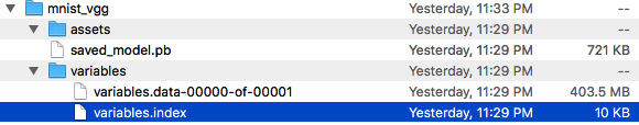
Figure 8.6 – Size of the trained VGG-16 model for the MNIST dataset

In this section, we have discussed some technical approaches and ideas for the two-phase prediction pattern. We have discussed different combinations of phase one and phase two models to set up the two-phase prediction pattern. In the next section, we will discuss some use cases of the two-phase model serving pattern.

Use cases of two-phase model serving

In this section, we will discuss some example cases where two-phase model serving can be used.

Case 1 – a fitness tracking device

Imagine that there is an app on our handheld device that recommends fitness tasks based on our activity. The device will go offline due to the absence of the network in a remote area or due to a poor signal. In that case, the device can’t make the API calls to the remote server to get recommendations. Therefore, we need a model deployed on the device that will be smaller than the model on the server. This small model will serve as the phase one model. A fitness tracker device can collect different features and use those features to get detailed recommendations from the server. However, the phase one model can only use a few critical features denoting whether the blood oxygen level is low, whether the heart rate is abnormal, whether the user has had enough rest, and so on. Based on these critical features, the device can then provide critical recommendations on whether the user needs to rest, drink water, and so on. The device can check the network strength whenever a recommendation needs to be made. If the network is weak, the device will ask the phase one model to make recommendations, and if the network is strong, the device will make an API call to get recommendations from the phase two model on the server.

Case 2 – a location with low internet speed

The internet is slow in many countries. In this scenario, we can’t keep calling the APIs on the server all the time to get predictions. We need to use the offline model on the device to avoid making API calls. In that case, we have to update the offline phase one model frequently. We can use both the phase two model and the phase one model to make predictions and then compute the error. We can use this error to improve the phase one model and also to provide an error estimation to the user with respect to the phase two model. For example, here are some dummy predictions from the phase one and phase two models:

Figure 8.7 – Predictions from the phase one and phase two models for some dummy samples

Now we can compute the median or average deviation from all the deviations in the last column and then use that metric, along with the predictions from the phase one model, to provide error estimates to the users.

For example, we can compute the median and average deviations using the following code snippet:

import numpy as np
deviations = np.array([7.69, 6.67, 5.88, 5.26, 4.76])
med_deviations = np.median(deviations)
print(med_deviations)
avg_deviations = np.average(deviations)
print(avg_deviations)

We get the following output:

5.88
6.052

Whenever we provide predictions from the phase one model, the predictions can be tagged with these error estimates. For example, if the model predicts 6, we can state that the prediction is likely to have a deviation of 6.052%, the average deviation. So, the most likely actual value is as follows:

6 / (100 – 6.052)% = 6 / 0.93948 ~ 6.39

Interestingly, 6.39 is closer to the value of 6.5 predicted by the phase two model.

The high-level strategy of combining the predictions from the phase one model and the error estimation model is shown in Figure 8.8:

Figure 8.8 – Combining the predictions from the phase one model and the error estimator model to get a more accurate prediction

In Figure 8.8, we have two models. The Phase one model and the Error estimation model both are passed the same input. The Error estimation model is trained using the deviation in prediction data in Figure 8.7. The predictions from the models are combined inside the Combiner block, and we get the final prediction Y, which is expected to be closer to the phase two prediction model.

Case 3 – weather forecasts

For weather forecasts from apps on edge devices, we might have to depend on the offline phase one model to get an estimated prediction of the weather. In this case, the phase one forecasting model will use features tracked using sensors on the device. For example, we can collect features such as air temperature, wind speed, luminosity, and humidity. The phase one model can be created to use only these critical features. On the other hand, the phase two model can use features from weather stations as well as features from edge devices.

Case 4 – route planners

We use edge devices to make route planners for our journeys. We want these apps to provide recommendations even if the network is offline. A phase one model may be used to provide the best possible offline route. This phase one model might not be able to consider live information on congestion, crashes, and so on. However, it can use some primary basic features such as distance, geolocation, source location, and destination location to provide a route to the destination, so that you do not get lost in remote locations where the network is very weak.

Case 5 – smart homes

In smart homes, we can have devices that set the room temperature, start sprinklers, turn on air conditioning, and so on. In these cases, we can have two different models. The first model will listen to the basic queries that will enable the default service or turn off the service.

For example, for commands such as the following, we can use a phase one model:

• Turn on the light
• Turn off the light
• Turn on the fan
• Turn off the fan
• Turn on the air conditioning
• Turn off the air conditioning

These commands can be addressed even by a simple model that can make binary YES/NO binary decisions.

Now let’s consider the following detailed commands that need more complex analysis:

• Turn on the light in the master bedroom
• Turn on the light in bathroom one
• Turn on the AC and set the temperature to T
• Turn on the fans in the living room

These commands can’t be handled easily by the small phase one model. So, we can redirect the prediction of these commands to the phase two model deployed in the cloud.

In this section, we have discussed some use cases of two-phase model serving. Besides the use cases described here, there are many other use cases where two-phase model serving should be chosen as the best option.

Summary

In this chapter, we have discussed two-phase model serving. We have explained what two-phase model serving is and why it is needed. We have also discussed different combinations of phase one and phase two models. We have seen that the phase one model can be created via quantization of the phase two model, which involves training only a single model. The phase one model can also be trained separately from the phase two model. These techniques are discussed along with some basic examples throughout the chapter. We have also discussed some examples of two-phase model serving.

In the next chapter, we will talk about the pipeline pattern. We will learn how ML pipelines are created, how different stages in the pipeline are interconnected to serve the model, and how the execution of the pipeline is scheduled.

Further reading

• To find out more about TensorFlow Lite, visit https://www.tensorflow.org/lite
• To find out more about model optimization and quantization techniques, visit https://www.tensorflow.org/lite/performance/model_optimization
• To find out more about the VGG-16 model for MNIST, visit https://www.kaggle.com/code/chandraroy/vgg-16-mnist-classification