9

Pipeline Pattern Model Serving

In this chapter, we will discuss the pipeline pattern of model serving. In this pattern, we create a pipeline with a number of stages. In each of the stages, some functionalities (such as data collection and feature extraction) are performed. The pipeline is started using a scheduler or it can be started manually. We will discuss how to create a pipeline for serving machine learning (ML) models and demonstrate how the pipeline pattern can be used for this purpose. The high-level topics that will be covered in this chapter are as follows:

• Introducing the pipeline pattern
• Introducing Apache Airflow
• Demonstrating a machine learning pipeline using Apache Airflow
• Advantages and disadvantages of the pipeline pattern

Technical requirements

In this chapter, we will use Apache Airflow to demonstrate pipeline creation via the pipeline pattern. For all the resources, documentation, and tutorials on Apache Airflow, please visit their website: https://airflow.apache.org/. We will give a high-level overview of Apache Airflow and how to use it to create pipelines, but we will not cover details of the Apache Airflow infrastructure. Feel free to learn more about Apache Airflow to see how to create complex pipelines and workflows. Please install Apache Airflow following the instructions for your OS on their official website.

All the code for this chapter is provided at https://github.com/PacktPublishing/Machine-Learning-Model-Serving-Patterns-and-Best-Practices/tree/main/Chapter%209.

If you get ModuleNotFoundError while trying to import any library, then you should install that module using the pip3 install <module_name> command.

Introducing the pipeline pattern

In the pipeline pattern, we create a pipeline to serve an ML model. Instead of all the steps of an ML pipeline happening in a central place, the steps are separated to occur in different stages of a pipeline. A pipeline is a collection of a number of stages in the form of a directed acyclic graph (DAG). We will start by describing DAGs in the following subsection and then gradually describe how the pipeline is formed by connecting different stages as a DAG.

A DAG

A DAG is a graph where the vertices are connected by directed edges, and no path in the graph forms a cycle. A path is a sequence of edges in a graph. A path forms a cycle if the start and end nodes of the path are the same. The directions of the edges are denoted by arrows. Nodes in the DAG are represented by circles. To understand DAGs graphically, let’s see a few graphs that are not DAGs.

First of all, let’s look at the graph in Figure 9.1. This graph is not a DAG as one of the edges of this graph, AC, does not have a direction.

Figure 9.1 – A non-DAG as the edge AC does not have a direction

Therefore, the presence of direction in a graph is a key requirement for the graph to be a DAG. This is evident from the name of this kind of graph. The letter D denotes Directed, which can help you to remember that the edges in the graph will have direction.

Now let’s look at the graph in Figure 9.2. In this graph, again, all the edges have direction. However, the graph is still not a DAG.

Figure 9.2 – A non-DAG due to the presence of a cyclic path, CBD

The second letter A in DAG denotes Acyclic, which means there can’t be any cyclic paths in the graph. The graph in Figure 9.2 has a cyclic path, CBD, which is colored red in the figure. Due to the presence of this cyclic path, the graph in Figure 9.2 is not a DAG. In this subsection, we have discussed some concepts on DAG. In the next subsection, we will discuss the stages of the pipeline and how a stage can be represented as a node in the DAG.

Stages of the machine learning pipeline

A stage of a pipeline is like a node in a graph. In these stages, a unit of activity happens. We can split the bigger task of the end-to-end process of serving the ML model, starting with data collection, into multiple steps as follows:

1. Data collection: In this stage, we collect data for the ML model from different data sources. We can collect data from surveys, sensors, social media posts, and so on.
2. Data cleaning: After collecting the data, we need to do some cleaning of the data to make it usable in the program. The data cleaning process can involve some manual operations as well as using some built-in functions and tools.
3. Feature extraction: In this step, we extract the features from the cleaned data to be used for training the model.
4. Training the model: After the feature extraction, we can train the model using those features. If we need more data or more features we can go back to the previous stages.
5. Testing the model: After the model is trained, we test the performance of the model with some unseen data.
6. Saving the model: After the testing is done and we are happy with the performance of the model, we can save the model for deploying or serving.

Note

Please note that here serving is not decoupled from the pipeline. However, the main goal of serving is to provide customers with access to the model’s response, usually from the last stage of the pipeline. We can take the prediction created from the prediction stage directly or create some REST APIs to access the predictions.

The pipeline is the connection of stages in the form of a DAG. The graph needs to be acyclic because we do not want to get lost in a loop inside the pipeline. If a cyclic path exists in the pipeline, then there is a chance that the pipeline will keep looping through that cyclic path. Therefore, we will use a DAG to create the pipeline. Using a DAG will ensure the following things:

• The directions of the edges will provide clear guidelines on how to move forward from a stage
• Acyclic paths will ensure that our program does not get trapped in a never-ending loop

In this section, we have learned about the pipeline pattern, DAGs, and how DAGs can be used to create pipelines via the pipeline pattern. In the next section, we will introduce you to Apache Airflow.

Introducing Apache Airflow

In this section, we will give you a high-level overview of Apache Airflow. To find out more details about Apache Airflow, read the documentation on their official website. The link to the official website is provided in the Technical requirements section.

Getting started with Apache Airflow

Apache Airflow is a full stack platform for creating workflows or pipelines using Python, scheduling the pipeline, and also monitoring the pipeline using the GUI dashboard provided by the platform. To see the tool on your local machine and understand how to create a pipeline, please install Apache Airflow. I am showing the steps I used to install Apache Airflow on macOS:

1. To install Apache Airflow, first, create a directory on your local machine and set the AIRFLOW_HOME variable. This is important because Apache Airflow will install the configurations here and fetch the workflows from this directory. I created a directory on my desktop and exported the AIRFLOW_HOME path using the following command from the terminal:

   export AIRFLOW_HOME=/Users/mislam/Desktop/airflow-examples
2. Then, you can install Apache Airflow using the following command:

   pip install "apache-airflow[celery]==2.3.4" --constraint "https://raw.githubusercontent.com/apache/airflow/constraints-2.3.4/constraints-3.7.txt"

You can also install Apace Airflow in a virtual environment instead of on your own platform. Follow the instructions on the installation page, https://airflow.apache.org/docs/apache-airflow/stable/installation/index.html, to get detailed instructions on installation to your appropriate device.

3. Then we confirm whether the installation was successful by typing the following command:

   $ airflow version

You should see the version number of Apache Airflow on the terminal. You can then go to the directory, which is set as AIRFLOW_HOME, and see some files created for you, as shown in Figure 9.3. You will not see a dags folder at the beginning. This is because you need to create it manually.

Figure 9.3 – Apache Airflow created installation files

We have to create the dags folder manually and place all the DAGs in it. To understand why we need to place all the DAGs in this folder, open the airflow.cfg file and find out the value for the dags_folder variable, as shown in Figure 9.4. Airflow fetches the DAGs from this folder. If you need to place DAGs from a different folder, you can change this path.

Figure 9.4 – The value of the dags_folder variable in the airflow.cfg file

Therefore, whenever we want to run a workflow and monitor it using the GUI, we need to place it inside the $AIRFLOW_HOME/dags folder.

Then, in the terminal, we run the following command to initialize the Airflow database that will be used to keep track of the users and the workflows:

airflow db init

4. Then, we need to create an Admin user to log in to the Airflow UI. We can create a dummy user using the following command:

   airflow users  create --role Admin --username admin --email admin --firstname admin --lastname admin --password admin

Feel free to change the information if you want. We use the dummy values to get access to the UI for demonstration purposes.

Creating and starting a pipeline using Apache Airflow

After Apache Airflow is installed successfully, we can create workflows and see whether it is working:

1. Now, let’s create a basic workflow using the following code snippet:

   # The DAG object; we'll need this to instantiate a DAG

   from datetime import datetime, timedelta

   from airflow import DAG

   from airflow.operators.bash import BashOperator

   with DAG(

       'example_tutorial',

       default_args={

           'depends_on_past': False,

           'email': ['[email protected]'],

           'email_on_failure': False,

           'email_on_retry': False,

           'retries': 1,

           'retry_delay': timedelta(minutes=5)

       },

       description='A simple tutorial DAG',

       schedule_interval=timedelta(days=1),

       start_date=datetime(2022, 1, 1),

       catchup=False,

       tags=['dummy'],

   ) as dag:

       # t1, t2 examples of tasks created by instantiating operators

       t1 = BashOperator(

           task_id='stage1',

           bash_command='python3 /Users/mislam/Desktop/airflow-examples/dags/stage1.py',

       )

       t2 = BashOperator(

           task_id='stage2',

           bash_command=' python3 /Users/mislam/Desktop/airflow-examples/dags/stage2.py',

       )

       t1 >> t2

In this code snippet, we first create a DAG using the DAG class provided by Airflow. We set the id of the DAG to example_tutorial. We also pass other properties, such as tags = ['dummy'], schedule_interval = timedelta(days=1), and so on. Using tags, we can search the workflow from the dashboard, as shown in Figure 9.7.

Then, we use BashOperator (provided by Airflow) to create a stage in the pipeline. According to Airflow terminology, stages are known as tasks. We create two tasks, t1 and t2, with IDs of stage1 and stage2, respectively. In the first stage, we run a Python file, stage1.py, and in the second stage, we run another Python file, stage2.py.

The stage1.py file contains the following code snippet:

import time
print("I am at stage 1")
time.sleep(5)
print("After 5 seconds I am existing stage 1")

And the stage2.py file contains the following code snippet:

print("I am at stage 2")

2. Now, we place stage1.py and stage2.py along with the file containing the DAG in the $AIRFLOW_HOME/dags directory.
3. Then we have to start airflow scheduler. This scheduler takes care of loading the new workflows to the UI, starting workflows when scheduled, and so on. We can start the scheduler using the following command:

   airflow scheduler
4. Then, let’s start the Airflow web server using the following command:

   airflow webserver

We should see that the web server has been started, as shown in Figure 9.5:

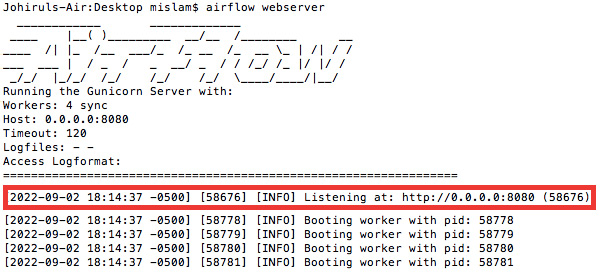
Figure 9.5 – The Airflow web server has been started and is listening at http://0.0.0.0:8080 or http://localhost:8080

5. Let’s open a browser and visit http://localhost:8080/, and we will see the screen shown in Figure 9.6:

Figure 9.6 – The Sign In screen of the Airflow UI launched after visiting the URL http://localhost:8080/

6. After the Sign In screen appears, we have to enter the admin username and password that we created in the last sub-section. After successfully signing in, we will see a home screen with a list of workflows, as shown in Figure 9.7:

Figure 9.7 – List of workflows shown in the Airflow UI after signing in

7. We see the option to search the workflows in the two text boxes above the list. Let’s filter the workflow by our dummy tag, and click on the DAG ID. It will take us to the page showing the details about the workflow. The workflow or pipeline is shown in Figure 9.8:

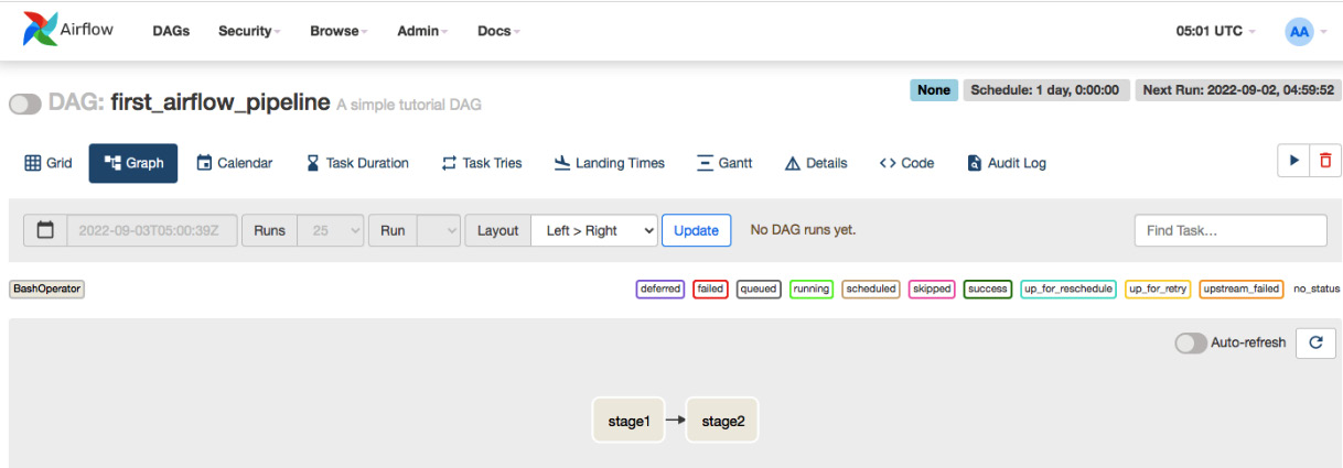
Figure 9.8 – Detailed view of the workflow first_airflow_pipeline

The home page of the workflow has a lot of information. You can view the history of runs, the next run time, the logs, the graphical representation of the pipeline, and more. For example, in our example, we created a pipeline with two stages, stage1 and stage2. We see the pipeline on the dashboard, along with the direction of connection between the edges. This direction is specified in the code. In our code, we created the pipeline and specified the direction from stage1 to stage2 via t1 >> t2 in the following code snippet:

t1 = BashOperator(
        task_id='stage1',
        bash_command=' python3 /Users/mislam/Desktop/airflow-examples/dags/stage1.py',
    )
    t2 = BashOperator(
        task_id='stage2',
        bash_command=' python3 /Users/mislam/Desktop/airflow-examples/dags/stage2.py',
    )
    t1 >> t2

If we want to reverse the direction, then we have to replace t1 >> t2 with t2 >> t1. The >> or << operator, which looks like an arrowhead, gets converted to an arrow in the pipeline, and the operator direction is the same as the direction of the arrow.

8. Now, we see in the top-right corner of the workflow in Figure 9.8 that the workflow will run daily at a specified time. We can also write more complex cron jobs to schedule the workflow. In that case, the field will take a cron expression as a string, such as schedule_interval="<cron expression>". We discussed cron expressions in Chapter 6, Batch Model Serving. To find out more about scheduling, visit https://airflow.apache.org/docs/apache-airflow/1.10.1/scheduler.html. However, we can also manually start the workflow any time we want. Let’s click the blue start button, as shown in Figure 9.9, and then click the Trigger DAG option.

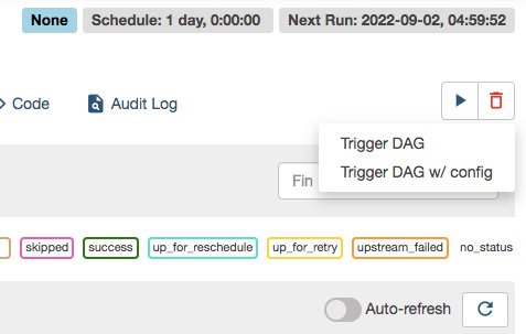
Figure 9.9 – Button to start the workflow manually

After both stages have finished running, we will see that the border of both stages has turned green, as shown in Figure 9.10. The legends above the Auto-refresh button show the meaning of the different border colors.

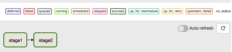
Figure 9.10 – All the stages of the pipeline completed

Later stages in the pipeline can only start after the previous stages have finished successfully. You can see this change of color interactively in the UI. For example, in our pipeline, stage2 will only start after stage1 is finished. We can confirm this by looking at the log. Let’s click on stage1 of the pipeline, and we will see a pop-up window, as shown in Figure 9.11:

Figure 9.11 – Pop-up window appears after clicking stage1 from which we can see the logs and execution history

By clicking the Log button, we can see the stage1 log and note the following two lines from the log, which prints the following output from the code in the stage1.py Python file that is being run inside stage1:

[2022-09-03, 06:00:07 UTC] {subprocess.py:92} INFO - I am at stage 1
[2022-09-03, 06:00:07 UTC] {subprocess.py:92} INFO - After 5 seconds I am existing stage 1

Similarly, we check the stage2 log and note the following line, which prints the output from the code in the stage2.py Python file, which is run inside stage2:

[2022-09-03, 06:00:12 UTC] {subprocess.py:92} INFO - I am at stage 2

From the highlighted times of the logs from the two stages, we can see that the output of stage2 was generated after the execution of stage1 completed. So, we have evidence that a later stage in the directional path starts only after the previous stages are complete.

In this section, you were introduced to Apache Airflow and installed it, and saw how to view the pipelines using the Airflow UI, how to run a pipeline, and how to view the output. In the next section, we will create a dummy ML pipeline using Airflow and see how to create a pipeline to serve an ML model following the pipeline pattern.

Demonstrating a machine learning pipeline using Airflow

In this section, we will create a dummy ML pipeline. The pipeline will have the following stages:

• One stage for initializing data and model directories if they are not present
• Two stages for data collection from two different sources
• A stage where we combine the data from the two data collection stages
• A training stage

You can have multiple stages depending on the complexity of your end-to-end process. Let’s take a look:

1. First, let’s create the DAG using the following code snippet:

   with DAG(

       'dummy_ml_pipeline',

       description='A dummy machine learning pipeline',

       schedule_interval="0/5 * * * *",

       tags=['ml_pipeline'],

   ) as dag:

       init_data_directory >> [data_collection_source1, data_collection_source2] >> data_combiner >> training

In the preceding code snippet, we created a pipeline by connecting the tasks or stages using init_data_directory >> [data_collection_source1, data_collection_source2] >> data_combiner >> training. Between the first and second >> operators, we have passed a list of two stages. This means that the data_combiner stage will only start if both the data_collection_source1 and data_collection_source2 stages are complete. It will be clearer if we look at the pipeline in the UI, as shown in Figure 9.12:

Figure 9.12 – A dummy pipeline with multiple dependencies

In the code snippet, we have omitted some of the parameters from the constructor that are the same as the pipeline we created before. We have changed the id, description, schedule_interval, and tags parameters of the DAG. The schedule_interval parameter is now given a "0/5 * * * *" cron expression. The meaning of this cron expression is that the cron job will run every 5 minutes and start the pipeline. This is how we can schedule our pipeline to run automatically at a certain time interval.

2. These stages are created using the following code snippet with BashOperator:

   init_data_directory = BashOperator(

           task_id='init_data_dir',

           bash_command='python3 /Users/mislam/Desktop/airflow-examples/dags/stages/init_data_dir.py',

       )

       data_collection_source1 = BashOperator(

           task_id='data_collection_1',

           bash_command='python3 /Users/mislam/Desktop/airflow-examples/dags/stages/data_collector_source1.py',

       )

       data_collection_source2 = BashOperator(

           task_id='data_collection_2',

           bash_command='python3 /Users/mislam/Desktop/airflow-examples/dags/stages/data_collector_source2.py',

       )

       data_combiner = BashOperator(

           task_id='data_combiner',

           bash_command='python3 /Users/mislam/Desktop/airflow-examples/dags/stages/data_combiner.py',

       )

       training = BashOperator(

           task_id='training',

           bash_command='python3 /Users/mislam/Desktop/airflow-examples/dags/stages/train.py',

       )

Note

You may notice that in these operators, we are using the path to different files and codes from the machine used to write these codes. You will have to change these paths based on the locations on your own machine. The same suggestion applies to all the examples we are using throughout the chapter.

3. These stages just run different Python files. The Python files contain dummy operations. For example, the init_data_dir.py file contains the following code:

   import os

   if not os.path.exists("/Users/mislam/Desktop/airflow-examples/dags/stages/data"):

       os.mkdir("/Users/mislam/Desktop/airflow-examples/dags/stages/data")

       print("The directory data is created")

   if not os.path.exists("/Users/mislam/Desktop/airflow-examples/dags/stages/model_location"):

       os.mkdir("/Users/mislam/Desktop/airflow-examples/dags/stages/model_location")

       print("The directory model_location is created")

It creates two directories, data, and model_location, for storing the data and model respectively in later stages.

The data_collector_source1.py file contains the following code snippet:

import pandas as pd
df1 = pd.DataFrame({"x": [2, 2, 2, 3, 4, 5], "y": [1, 1, 1, 1, 1, 1]})
df1.to_csv("/Users/mislam/Desktop/airflow-examples/dags/stages/data/data1.csv")

So, we write some dummy data in a CSV file in this code. We do a similar thing in the data_collector_source2.py file. In this file, we combine the data from these two data collection stages and write the combined data to a CSV file. In the training stage, we train a LogisticRegression model and save the trained model to the model_location folder created in the first stage.

4. We can wait till the pipeline finishes and then check that the data and model_location folders have been created and that the model has been saved in the model_location folder, as shown in Figure 9.13:

Figure 9.13 – Model is saved successfully after the execution of the pipeline is finished

We have saved this model to our local directory. We can save it inside a server, which will be used by the APIs, and we can create a prediction API to use the model for prediction.

5. To confirm whether the pipeline is scheduled to run every 5 minutes, let’s go to the Airflow UI and look at the scheduling information in the top-right corner. The scheduling information of our pipeline is shown in Figure 9.14:

Figure 9.14 – The pipeline is scheduled to run every 5 minutes using a cron expression

In this section, we have seen how to create an ML serving pipeline using Apache Airflow. In the next section, we will see some advantages and disadvantages of the pipeline pattern.

Advantages and disadvantages of the pipeline pattern

In this section, we will explore some of the advantages and disadvantages of the pipeline pattern.

First of all, the advantages of the pipeline pattern are as follows:

• We can split different critical operations of the end-to-end ML processes into the stages of a pipeline. Therefore, if a particular stage fails, we can fix that stage and restart the pipeline from there instead of starting from scratch. If you click on a pipeline stage, you will see that there is an option to start that stage without running the previous stages. You can use the Run button shown in Figure 9.11 to start a pipeline from a particular stage.
• You can monitor the pipeline using a UI and create pipelines with different structures using the operators provided by Apache Airflow.
• You can schedule the pipeline using the options provided by Apache Airflow, and thus, the pipeline can easily be run periodically to get the most up-to-date model.
• You can integrate pipelines with web servers to provide client APIs. You can save the model to a location that is referenced by the web server. In this way, you can avoid uploading the model to the server after the training is complete.

The advantages mentioned here make the pipeline pattern a very good option to choose if the ML application we want to deploy has a lot of stages.

Some of the disadvantages of the pipeline pattern are as follows:

• We need to be careful when setting up dependencies among the stages. For example, let’s assume stage s1 collects data for training and another stage, s2, uses the data collected by s1. We need to have s1 before s2 in the pipeline. If we somehow miss these dependencies, our pipeline will not work.
• Maintaining the pipeline server adds additional technical overhead. A team that needs to use the pipeline pattern might need a dedicated engineer who is an expert on the tool used to create pipelines.

In this section, we have seen some of the advantages and disadvantages of the pipeline pattern. In the next section, we will summarize the chapter and conclude.

Summary

In this chapter, we explored the pipeline model serving pattern and discussed how DAGs can be used to create a pipeline. We have also covered some fundamental concepts on DAG to help you understand what DAGs are.

Then we introduced a tool called Apache Airflow, which can be used to create pipelines. We saw how to get started with Apache Airflow and how to use the operators provided by Apache Airflow to create a pipeline. We saw how dependencies are created using Apache Airflow and how to create separate stages using separate Python files.

We then created a dummy ML pipeline for collecting and combining data, training a model using the data, and then saving the model to a location that is accessible by the server. We explored how to create many-to-one dependencies among the stages for when a stage’s actions depend on the completion of multiple stages.

Finally, we discussed the advantages and disadvantages of the pipeline pattern. In the next chapter, we will discuss the ensemble pattern. We will see how multiple models can be combined and served.

Further reading

• You can read about Apache Airflow at https://airflow.apache.org/docs/
• You can learn about the Apache Airflow scheduler at https://airflow.apache.org/docs/apache-airflow/stable/concepts/scheduler.html
• To find out more about DAGs, you can visit https://bookdown.org/jbrophy115/bookdown-clinepi/causal.html