13

Using Ray Serve

In this chapter, we will talk about serving models with Ray Serve. This is one of the most popular tools for serving ML models. It is a framework-agnostic scalable model-serving library. ML models created using almost any library can be served using Ray Serve. We will explore this library in this chapter and show some hands-on examples to get you up and running with Ray Serve. Covering all the topics and concepts of Ray Serve itself would demand a separate book. So, we will just cover some basic information and the end-to-end process of using Ray Serve.

At a high level, we are going to cover the following main topics in this chapter:

• Introducing Ray Serve
• Using Ray Serve to serve a model

Technical requirements

In this chapter, we will mostly use the same libraries that we used in the previous chapters. You should have Postman or another REST API client installed to be able to send API calls and see the response. All the code for this chapter is provided at https://github.com/PacktPublishing/Machine-Learning-Model-Serving-Patterns-and-Best-Practices/tree/main/Chapter%2013.

If you get ModuleNotFoundError while trying to import any library, then you should install that module using the pip3 install <module_name> command. In this chapter, you will need to install Ray Serve. Please use the pip3 install "ray[serve]" command to do so.

Introducing Ray Serve

Ray Serve is a framework-agnostic model-serving library. It is scalable and creates inference APIs on your behalf. Some of the key concepts in Ray Serve are as follows:

• Deployment
• ServeHandle
• Ingress deployment

We will look at each of these in the following sections.

Deployment

A deployment contains the business logic and the ML model that will be served. To define a deployment, the @serve.deployment decorator is used. For example, let’s take a look at the following code snippet, which shows a very basic deployment that will return whatever message is passed by the user as a payload:

@serve.deployment class MyFirstDeployment:  # Take the message to return as an argument to the constructor.  def __init__(self, msg):      self.msg = msg   def __call__(self):      return self.msg my_first_deployment = MyFirstDeployment.bind("Hello world!")

In this code snippet, we define the MyFirstDeployment deployment using the @serve.deployment decorator. This class has the __call__ method, which is invoked whenever we hit the endpoint from the server. We can see that this method returns whatever message is passed while creating the instance of the deployment. For example, we can create a deployment instance using the following code snippet:

my_first_deployment = MyFirstDeployment.bind("Hello world!")

Now, we can serve the deployment using the following command:

serve run first_ray_serve_demo:my_first_deployment

Here, first_ray_serve_demo is the name of the Python file with the .py extension.

After running this command, we will see the following log:

2022-10-16 08:31:24,992 INFO scripts.py:294 -- Deploying from import path: "first_ray_serve_demo:my_first_deployment".
2022-10-16 08:31:30,687 INFO worker.py:1509 -- Started a local Ray instance. View the dashboard at 127.0.0.1:8265 
(ServeController pid=58356) INFO 2022-10-16 08:31:34,636 controller 58356 http_state.py:129 - Starting HTTP proxy with name 'SERVE_CONTROLLER_ACTOR:SERVE_PROXY_ACTOR-9080e55fa7ae17885d254728a191fb44766ea3105cd0c63fb624e6bd' on node '9080e55fa7ae17885d254728a191fb44766ea3105cd0c63fb624e6bd' listening on '127.0.0.1:8000'
(ServeController pid=58356) INFO 2022-10-16 08:31:35,674 controller 58356 deployment_state.py:1232 - Adding 1 replicas to deployment 'MyFirstDeployment'.
(HTTPProxyActor pid=58369) INFO:     Started server process [58369]

Let’s look at the highlighted portions of the code. From the first highlighted part of the log, we notice that a dashboard is created where we can see the local instance that is running. If we go to 127.0.0.1:8265, we will see a dashboard showing all the active nodes, as shown in Figure 13.1:

Figure 13.1 – Ray dashboard showing all the active nodes

From this figure, we notice that an active node with an ID starting with 908 is running the HTTP proxy. We also notice that a replica for our deployment, ray::ServerReplica:MyFirstDeployment, is running. From the log, we notice that the server is listening to the HTTP requests on 127.0.0.1:8000. Let’s go to that endpoint from Postman. We will see the following response in Postman:

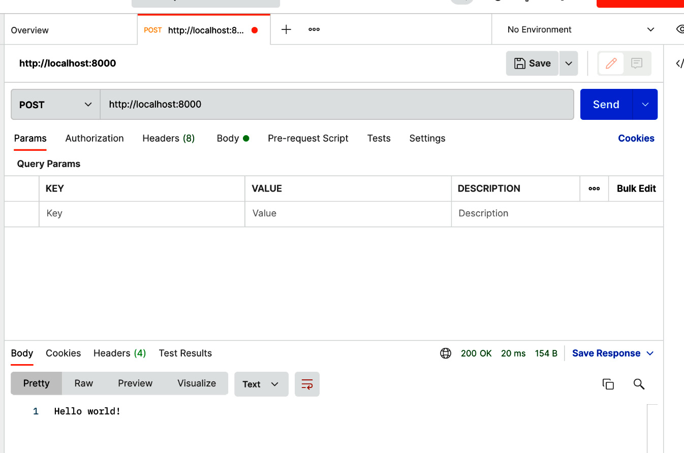
Figure 13.2 – Postman response from MyFirstDeployment ServerReplica

We got the response Hello World! because this is what we passed when creating the deployment instance in our code. We did not provide an option to pass the payload from the HTTP request.

ServeHandle

ServeHandle is a reference to a running deployment. If we call the remote method on ServeHandle, then we get the same response that we would get using an HTTP request. This allows us to smartly invoke the inference APIs from the program. Using ServeHandle, we can do a composite of multiple models. We can pass the models as ServeHandles during binding. For example, let’s consider the following code snippet:

import ray from ray import serve @serve.deployment class ModelA:    def __init__(self):        self.model = lambda x : x + 5     async def __call__(self, request):        data = await request.json()        x = data['X']        return self.model(x)@serve.deployment class ModelB:    def __init__(self):        self.model = lambda x : x * 2     async def __call__(self, request):        data = await request.json()        x = data['X']        return self.model(x)@serve.deployment class Driver:    def __init__(self, model_a_handle, model_b_handle):        self._model_a_handle = model_a_handle         self._model_b_handle = model_b_handle     async def __call__(self, request):        ref_a = await self._model_a_handle.remote(request)        ref_b = await self._model_b_handle.remote(request)        return (await ref_a) + (await ref_b)model_a = ModelA.bind()model_b = ModelB.bind()driver = Driver.bind(model_a, model_b)

In this code snippet, we have two models, ModelA and ModelB. These models just contain dummy computations for now. ModelA takes x as input and returns x + 5. ModelB takes x as input and returns 2*x. Now, note that we are using another deployment called Driver, where we are passing both ModelA and ModelB after binding. These models are passed as ServeHandles and can independently provide an HTTP response or a response using the remote() function. Now, let’s run the program using the following command in the terminal:

serve run model_composition:driver

Now, we can take a look at the log of the model deployment to understand what is happening. I have taken the following snippet of the log to show that Ray Serve has created a separate deployment for each of the deployments:

(ServeController pid=94883) INFO 2022-10-16 15:40:12,999 controller 94883 deployment_state.py:1232 - Adding 1 replicas to deployment 'ModelA'.
(ServeController pid=94883) INFO 2022-10-16 15:40:13,019 controller 94883 deployment_state.py:1232 - Adding 1 replicas to deployment 'ModelB'.
(ServeController pid=94883) INFO 2022-10-16 15:40:13,034 controller 94883 deployment_state.py:1232 - Adding 1 replicas to deployment 'Driver'.

Here, we have passed the ServeHandles for ModelA and ModelB to the driver. Inside the driver, we can make HTTP calls to the ServeHandles using the following snippet:

 ref_a = await self._model_a_handle.remote(request) ref_b = await self._model_b_handle.remote(request)

Now, we can make a request from Postman and see the output, as shown in Figure 13.3:

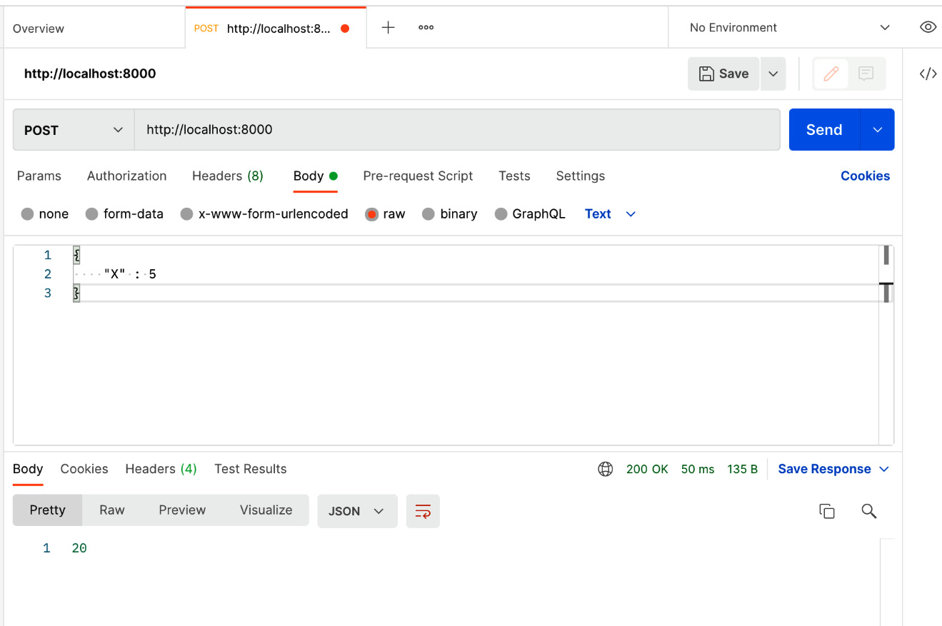
Figure 13.3 – Example of making HTTP calls to a deployment with model composition

We got an output of 20 by passing the input, {"X": 5}. Let’s see how we get this output:

• ModelA takes the input and returns 5 + 5 = 10
• ModelB takes the input and returns 2*5 = 10
• Driver takes the responses from both models and returns the addition of these results using return (await ref_a) + (await ref_b)

Therefore, we got 20. This idea of ServeHandles is to enable you to composite multiple models and effectively carry out model serving using the ensemble pattern.

Ingress deployment

When serving multiple models using model composition, there will always be a top-level deployment that will handle HTTP requests. For example, in the preceding code snippet, Driver takes care of handling the HTTP requests. It then calls other models in the composition using ServeHandles. This top-level deployment is called ingress deployment. Remember that everything with the @serve.deployment decorator is a deployment. Other deployments can be specific to particular models and they are passed to the ingress deployment as ServeHandles after binding using the bind() method.

Deployment graph

Ray Serve supports an API to form a graph of different deployments. Using this concept, we can compose multiple models in the form of a graph. This helps us serve an ML model using the pipeline pattern. For example, let’s look at the following code snippet, where we are creating a pipeline with four sequential steps. Each step of the pipeline just adds a suffix with the step name. This will help us understand in what order the steps in the graph are executed:

1. Use the following code snippet to create step 1 of the pipeline in the Step1 function:

   import ray from ray import serve from ray.serve.dag import InputNode from ray.serve.drivers import DAGDriver @serve.deployment def Step1(inp: str) -> str:    print("I am inside step 1")    return f"{inp}_step1"

The Step1 method will create the first step in the pipeline and will print a message stating I am inside step 1. It will also return a string ending with the _step1 suffix, indicating the output is coming from step 1 of the pipeline.

2. In this code snippet, we just added the _step1 suffix to the input. The program for step 2 of the pipeline is as follows:

   @serve.deployment def Step2(inp: str) -> str:    print("I am inside step 2")    return f"{inp}_step2"

The Step2 method will create step 2 of the pipeline. This step will print a message stating I am inside step 2 and return a string ending with the _step2 suffix.

3. This step adds the _step2 suffix to the input. The program for step 3 is as follows:

   
@serve.deployment def Step3(inp: str) -> str:    print("I am inside step 3")    return f"{inp}_step3"

Inside the Step3 function, we put the logic for step 3 of the pipeline. This step prints a message stating I am inside step 3 and returns a string ending with the _step3 suffix.

4. The program for step 4 is as follows:

   
@serve.deployment def Step4(inp: str) -> str:    print("I am inside step 4")    return f"{inp}_step4"

Step 4 adds the _step4 suffix to the input.

5. The model deployment can be created using the following class, which provides the prediction response. The predict method adds the _predict suffix to the input:

   @serve.deployment class Model:    def __init__(self):        self.model = lambda x : f"{x}_predict"    def predict(self, inp: str) -> str:        print("I am inside predict method")        return self.model(inp)with InputNode() as input:    model = Model.bind()    step1 = Step1.bind(input)    step2 = Step2.bind(step1)    step3 = Step3.bind(step2)    step4 = Step4.bind(step3)    output = model.predict.bind(step4)    serve_dag = DAGDriver.bind(output)handle = serve.run(serve_dag)print(ray.get(handle.predict.remote("hello")))

Now, if we run the program, we will get hello_step1_step2_step3_step4_predict as output. We can run it as many times as we want and we will get the same output. So, we got the idea that the steps in the graph or pipeline are executed in order. Following this technique, we can use the pipeline pattern to deploy the ML model.

In this section, we have provided a high-level overview of Ray Serve and discussed some key concepts, along with examples. In the next section, we will use Ray Serve to serve some models from end to end. First, we will use the composition of models to serve a model while following the ensemble pattern, and then use the concept of a deployment graph to deploy a model following the pipeline pattern.

Using Ray Serve to serve a model

In this section, we will use Ray Serve to serve two dummy models using the ensemble and pipeline patterns. We will use very basic models just to demonstrate the end-to-end process of using Ray Serve.

Using the ensemble pattern in Ray Serve

In this subsection, we will use Ray Serve to ensemble the results of two scikit-learn models:

1. First of all, let’s create a deployment for deploying a RandomForestRegressor model using the following code snippet:

   from ray import serve from sklearn.ensemble import RandomForestRegressor from sklearn.ensemble import AdaBoostRegressor from sklearn.datasets import make_regression @serve.deployment class RandomForestRegressorModel:    def __init__(self):        X, y = make_regression(n_features=4, n_informative=2,                               random_state=0, shuffle=False)        self.model = RandomForestRegressor(max_depth=2, random_state=0)        self.model.fit(X, y)    async def __call__(self, request):        data = await request.json()        x = data['X']        pred = self.model.predict(x)        print("Prediction from RandomForestRegressor is ", pred)        return pred

Note that inside the constructor we are training, the model is using dummy data. Ideally, you would need to import the model from persistent storage instead of training on the fly inside the constructor. We are using this dummy dataset for training as we just want to show how ensembling using Ray Serve works. In practice, to solve a real business problem, you need data from well-defined sources. We predicted with the input data inside the __call__ method. We also added a print statement to see the prediction from this model in the log.

2. Now, let’s create another deployment for serving the AdaBoostRegressor model with the following code snippet:

   @serve.deployment class AdaBoostRegressorModel:    def __init__(self):        X, y = make_regression(n_features=4, n_informative=2,                               random_state=0, shuffle=False)        self.model = AdaBoostRegressor(random_state=0, n_estimators=100)        self.model.fit(X, y)    async def __call__(self, request):        data = await request.json()        x = data['X']        pred = self.model.predict(x)        print("Prediction from AdaBoostRegressor is ", pred)        return pred

We follow the same style of training for this model as in step 1.

3. Next, let’s create a deployment to make a composition of the preceding two models by averaging the responses from them together, as shown in the following code snippet:

   @serve.deployment class EnsemblePattern:    def __init__(self, model_a_handle, model_b_handle):        self._model_a_handle = model_a_handle         self._model_b_handle = model_b_handle     async def __call__(self, request):        ref_a = await self._model_a_handle.remote(request)        ref_b = await self._model_b_handle.remote(request)        return ((await ref_a) + (await ref_b))/2.0

In this code snippet, we provided an argument in the constructor to pass two models as ServeHandles. These ServeHandles can be used to make an HTTP query to get responses from their models. This EnsemblePattern deployment is also known as an ingress deployment as it works as the client-facing deployment to handle HTTP requests.

4. Now, let’s provide the ingress deployment with two models as ServeHandles, as shown in the following code snippet:

   model_a = RandomForestRegressorModel.bind()model_b = AdaBoostRegressorModel.bind()ensemble = EnsemblePattern.bind(model_a, model_b)

We now have the ingress deployment ensemble ready to be deployed. Let’s save the full code inside a file named ensemble_example.py. We have to use the name of this file while serving the deployment.

5. Now, we can start running the deployment using the following command:

   serve run ensemble_example:ensemble

Here, ensemble_example is the name of the Python module and ensemble is the name of the ingress deployment. We will see the following log, indicating that the server has started and that the application is ready to take the request:

2022-10-16 21:53:15,083 INFO scripts.py:294 -- Deploying from import path: "ensemble_example:ensemble".
2022-10-16 21:53:18,589 INFO worker.py:1509 -- Started a local Ray instance. View the dashboard at 127.0.0.1:8265 
(ServeController pid=16220) INFO 2022-10-16 21:53:22,910 controller 16220 http_state.py:129 - Starting HTTP proxy with name 'SERVE_CONTROLLER_ACTOR:SERVE_PROXY_ACTOR-a650b61d63c7fade6fba77006da65d388b65d834b162db7dc7ac45b4' on node 'a650b61d63c7fade6fba77006da65d388b65d834b162db7dc7ac45b4'listening on '127.0.0.1:8000'
(HTTPProxyActor pid=16223) INFO:     Started server process [16223]
(ServeController pid=16220) INFO 2022-10-16 21:53:23,944 controller 16220 deployment_state.py:1232 - Adding 1 replicas to deployment 'RandomForestRegressorModel'.
(ServeController pid=16220) INFO 2022-10-16 21:53:23,962 controller 16220 deployment_state.py:1232 - Adding 1 replicas to deployment 'AdaBoostRegressorModel'.
(ServeController pid=16220) INFO 2022-10-16 21:53:23,976 controller 16220 deployment_state.py:1232 - Adding 1 replicas to deployment 'EnsemblePattern'.
2022-10-16 21:53:26,884 SUCC scripts.py:307 -- Deployed successfully.

I have highlighted a portion of the log indicating that for each of the deployments, a separate replica is created. They can now operate independently and can be composited in any combination. In this way, Ray Serve is a very efficient tool in supporting the ensemble pattern.

6. Now, we can test the inference API from Postman. Let’s send a request with [[0, 0, 0, 0]] as input. We will see the following output in the Postman response panel:

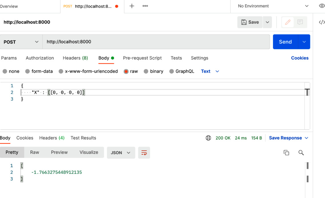
Figure 13.4 – Sending a request to the ensemble pattern model from Postman

Remember that we printed some logs from each of the deployments. Let’s go to the console to see these logs. We will see some new logs, such as the following, after the request is submitted from Postman:

(HTTPProxyActor pid=16223) INFO 2022-10-16 22:02:46,112 http_proxy 127.0.0.1 http_proxy.py:315 - POST / 200 1227.9ms
(ServeReplica:AdaBoostRegressorModel pid=16227) INFO 2022-10-16 22:02:46,109 AdaBoostRegressorModel AdaBoostRegressorModel#cxaWxB replica.py:482 - HANDLE __call__ OK 7.3ms
(ServeReplica:RandomForestRegressorModel pid=16226) INFO 2022-10-16 22:02:46,099 RandomForestRegressorModel RandomForestRegressorModel#AdWxyq replica.py:482 - HANDLE __call__ OK 8.5ms
(ServeReplica:AdaBoostRegressorModel pid=16227) Prediction from AdaBoostRegressor is  [4.79722349]
(ServeReplica:RandomForestRegressorModel pid=16226) Prediction from RandomForestRegressor is  [-8.32987858]
(ServeReplica:EnsemblePattern pid=16228) INFO 2022-10-16 22:02:46,110 EnsemblePattern EnsemblePattern#kHmkKI replica.py:482 - HANDLE __call__ OK 1220.7ms

The highlighted lines in the preceding logs show the predictions from the models. The prediction from AdaBoostRegressor is 4.79722349 and the prediction from RandomForestRegressor is –8.32987858. From the ingress deployment, we got the average of these two numbers as the final prediction – that is, (4.79722349 –8.32987858)/2 = -1.7663275448912135.

In this subsection, we showed you how to use Ray Serve to serve models using the ensemble pattern. In the next subsection, we will show you how to use Ray Serve to serve models using the pipeline pattern.

Using Ray Serve with the pipeline pattern

We discussed the pipeline pattern in Chapter 9. We can use the Ray Serve tool to serve models using the pipeline pattern. To use Ray Serve with the pipeline pattern, we need to use the concept of a deployment graph in Ray Serve, as we discussed previously.

We will create a pipeline by going through the following stages:

1. Data collection
2. Data cleaning
3. Feature extraction
4. Training
5. Predict

We will just use basic dummy operations in these steps to illustrate how the pipeline pattern works in Ray Serve. In the data collection stage, we will create a pandas DataFrame with some dummy data; in the data cleaning stage, we will do some basic cleaning to remove rows with missing data; in the feature extraction stage, we will convert the categorical data into numerical data using a built-in pandas method, and in the training stage, we will train a RandomForestRegression model with the features. Let’s get started:

1. First, let’s carry out the data collection step using the following code snippet:

   @serve.deployment def collect_data() -> pd.DataFrame:    df = pd.DataFrame({"F1": [1, 2, 3, 4, 5, None], "F2": ["C1", "C1", "C2", "C2", "C3", "C3"], "Y": [0, 0, 0, 1, 1, 1]})    print("DF in the data collection stage")    print(df)    return df

This step creates a dummy DataFrame. In models that serve real business problems, the data may come from databases, files, streaming data sources, and so on.

2. Note that in the data in step 1, there are some null values. We can carry out a basic data-cleaning step to remove these null values:

   @serve.deployment def data_cleaning(df: pd.DataFrame) -> pd.DataFrame:    df = df.dropna()    print("DF after the data cleaning stage")    print(df)    return df

This step returns the data after removing the rows that contain null values.

3. Now, let’s move on to a basic feature engineering step. In this step, we must encode the categorical values in the F2 column using the pandas.get_dummies API. The code snippet for this step is as follows:

   @serve.deployment def feature_engineering(df: pd.DataFrame) -> pd.DataFrame:    df = pd.get_dummies(df)    print("DF after the feature engineering stage")    print(df)    return df

After the cleaning, we return the modified DataFrame using return df so that the next stage in the pipeline can receive it. The next stage in the pipeline that will do model training depends on this data.

4. The fourth step is the training step. Usually, training is not part of the model-serving process, but in the pipeline pattern, it is embedded as a step in the pipeline. The main goal of serving is achieved from the previous step. So, let’s train a basic RandomForestRegressor model using the data passed from the previous step. The code snippet for this step is as follows:

   @serve.deployment def train(df: pd.DataFrame) -> RandomForestRegressor:    X = df[["F1", "F2_C1"]]    y = df["Y"]    print("Inside training!")    model = RandomForestRegressor(max_depth=2, random_state=0)    model.fit(X, y)    return model

This stage returns the model to the prediction by using return model after training. The prediction stage will be able to make predictions using the model provided by this training stage.

5. Then, we have the predict stage. In this stage, we take the model that comes from the training stage as input and also take an input, x, that is taken from an input node of the graph. We can use the following code snippet for the prediction step:

   @serve.deployment def predict(model: RandomForestRegressor, x) -> float:    print("Inside predict method")    print("Input is", x)    return model.predict(x)

After this prediction step is done, we can form a pipeline using the deployment graph concept of Ray Serve.

6. Now, let’s form the deployment graph by using the stages of the pipeline. The stages work as nodes of the graph; the connection that’s created between the stages using the bind function, as shown in the following code, works as edges. Note that each of the steps is a Ray Serve deployment with the @serve.deployment decorator:

   with InputNode() as input:    data_collection = collect_data.bind()    clean_data = data_cleaning.bind(data_collection)    feature_creation = feature_engineering.bind(clean_data)    train_model = train.bind(feature_creation)    output = predict.bind(train_model, input)    serve_dag = DAGDriver.bind(output)handle = serve.run(serve_dag)

The handle graph that was created via handle = serve.run(serve_dag) is now ready to run and make predictions. We can send a request from the Python program like so:

print(ray.get(handle.predict.remote([[1 , 1]])))

This line of code will make a prediction for the input of [[1, 1]] and print the prediction response from the model. After running the preceding program, we will see the following output in the console:

(ServeReplica:collect_data pid=66004) DF in the data collection stage
(ServeReplica:collect_data pid=66004)     F1  F2  Y
(ServeReplica:collect_data pid=66004) 0  1.0  C1  0
(ServeReplica:collect_data pid=66004) 1  2.0  C1  0
(ServeReplica:collect_data pid=66004) 2  3.0  C2  0
(ServeReplica:collect_data pid=66004) 3  4.0  C2  1
(ServeReplica:collect_data pid=66004) 4  5.0  C3  1
(ServeReplica:collect_data pid=66004) 5  NaN  C4  1

From the preceding log, notice that it just printed the DataFrame that we created and printed. The console log from the data cleaning step is as follows:

(ServeReplica:data_cleaning pid=66005) DF after the data cleaning stage
(ServeReplica:data_cleaning pid=66005)     F1  F2  Y
(ServeReplica:data_cleaning pid=66005) 0  1.0  C1  0
(ServeReplica:data_cleaning pid=66005) 1  2.0  C1  0
(ServeReplica:data_cleaning pid=66005) 2  3.0  C2  0
(ServeReplica:data_cleaning pid=66005) 3  4.0  C2  1
(ServeReplica:data_cleaning pid=66005) 4  5.0  C3  1

From the log in the data cleaning step, we can see that the row containing NaN is removed. The log from the feature engineering step is as follows:

(ServeReplica:feature_engineering pid=66006) DF after the feature engineering stage
(ServeReplica:feature_engineering pid=66006)     F1  Y  F2_C1  F2_C2  F2_C3
(ServeReplica:feature_engineering pid=66006) 0  1.0  0      1      0      0
(ServeReplica:feature_engineering pid=66006) 1  2.0  0      1      0      0
(ServeReplica:feature_engineering pid=66006) 2  3.0  0      0      1      0
(ServeReplica:feature_engineering pid=66006) 3  4.0  1      0      1      0
(ServeReplica:feature_engineering pid=66006) 4  5.0  1      0      0      1

Note that the data is encoded in the feature engineering step. We can also see features such as F2_C1, F2_C2, and F2_C3, which are created by pandas.get_dummies. The log from the training step is as follows:

(ServeReplica:train pid=66007) Inside training!

This is just a single line indicating that we have reached this step. The log from the predict method is as follows:

(ServeReplica:predict pid=66008) Inside predict method
(ServeReplica:predict pid=66008) Input is [[1, 1]]

This indicates that the input has been received correctly by the predict method.

The output from making the inference call through the print(ray.get(handle.predict.remote([[1 , 1]]))) print statement is as follows:

[0.02]

Therefore, we can see that the basic ML pipeline is working from end to end.

In this section, we have shown examples of using Ray Serve to serve ML models using the ensemble and pipeline patterns. Next, we will summarize this chapter and conclude.

Summary

In this chapter, we discussed Ray Serve. Ray Serve is a tool with a massive amount of features. Our goal was not to introduce everything about this tool in this chapter. Rather, we wanted to give you an introduction to the tool and outline the basic requirements to understand how this tool can be used in serving production-ready models while following different patterns of the serving model.

We provided an introduction to the key concepts of the tools, along with examples. We then used Ray Serve to serve two dummy models from end-to-end using the ensemble pattern and the pipeline pattern. Using these examples, we saw how Ray Serve can help you set up model serving while following the standard patterns of serving ML models.

In the next chapter, we will introduce you to BentoML, another tool for serving ML models.

Further reading

You can read the following articles to learn more about Ray Serve:

• To learn more about Ray Serve, check out the official documentation at https://docs.ray.io/en/latest/serve/index.html
• To learn more about the key concepts in Ray Serve, please use the following link: https://docs.ray.io/en/latest/serve/key-concepts.html