Chapter 8: Plug-In Charging Characteristics, Algorithm, and Impact on Power Distribution System

8.1 Introduction

During the last decade, PHEVs and BEVs have been developed in the marketplace. In addition to sharing the characteristics of traditional HEVs with two power sources, a PHEV/BEV is capable of driving miles in the pure electric mode, and the battery system can be recharged by a plug-in charger connected to the electric grid. Some PHEV/BEVs with a large battery system even can power the vehicle more than 40 miles so that daily commuters can potentially drive exclusively with the electric motor. The distinctions between HEVs and PHEVs are the all-electric driving mode and the plug-in charging capability from the electric grid.

With PHEVs and BEVs entering the marketplace, existing electric grids and power distribution systems may be impacted. To minimize the impact and achieve lowest charging cost for PHEV owners, plug-in charging strategies must be systematically studied, taking into consideration not only the capabilities of the battery system and plug-in charger but also the capability of the electric grid. The most recent results and current trends of control system and power electronic technology show that developing an optimal or smart plug-in charging control strategy is a realistic goal. This chapter will briefly introduce the plug-in charging characteristics and the impacts on the electric grid and distribution system as well as plug-in charging strategies.

8.2 Plug-in hybrid vehicle battery system and charging characteristics

As mentioned above, a PHEV can be driven specific number of miles purely on battery energy. To drive a midsize passenger vehicle 20–60 miles, the usable energy capacity of the battery system of a PHEV/BEV should be between 8 and 25 kWh. A PHEV normally uses the battery system in two modes: charge depleting (CD) and charge sustaining (CS). When the battery is operated in the CD mode, the vehicle is powered by the battery only; once the battery is drained to a specific level, the battery enters the CS mode where the vehicle is powered by the engine and battery system, and in this mode the power distribution from the engine and battery is determined by the energy management algorithm based on the states of vehicle and battery system. Furthermore, in the CS mode, the battery is principally utilized to provide short bursts of power with a powertrain and capture electric braking (regenerative) energy. The changing point from CD to CS is set based on the design targets, such as the service life of the battery system and the fuel economy, and the CS mode normally occurs between 20 and 30% SOC in a Li-ion battery system.

With plug-in charging, the amount of power charging to the battery is limited by the size of the wall electrical circuit and the capacity of the vehicle battery system, which consequently results in different plug-in charging time. Based on the AC voltage level and electrical circuit capacity, plug-in chargers are classified as 120 V AC and 240 V AC used in garages and rapid high-voltage DC charger for public service stations.

8.2.1 AC-120 Plug-In Charging Characteristics

An AC-120 plug-in charger is designed to charge a PHEV/BEV battery system, where the 120-V AC power outlet is available in a garage or parking lot. Since the electrical circuit in the garage is generally limited to 15A for a 120-V AC power outlet, the maximum charging power is normally designed up to 1.5 kW.

Due to the AC charging power limit, the charging current and time vary with the battery system used in a PHEV/BEV. For example, the charging characteristics of a PHEV battery system with 45 Ah capacity and supporting 40 electric miles can be obtained as follows:

Hybrid vehicle system design and calibration engineers need to know the charging current curve, terminal voltage curve, charging power curve, and SOC varying curve while the battery system is being charged by a plug-in AC charger from the given initial SOC to the final SOC. For example, when a Li-ion PHEV battery system with 45 Ah and 360 V nominal voltage is charged to 80% SOC from 30% SOC by an AC-120 charger, the corresponding charging curves are shown in Figs. 8.1, 8.2, 8.3, and 8.4. It takes 7.2 h for an AC-120 charger to charge the battery to the target SOC.

Figure 8.1 Current profile of PHEV battery system when charged by AC-120 charger.

Figure 8.2 Terminal voltage profile of PHEV battery system during charging by AC-120 charger.

Figure 8.3 SOC charging process of PHEV battery system when charged by AC-120 charger.

Figure 8.4 AC power charging profile.

8.2.2 AC-240 Plug-In Charging Characteristics

An AC-240 plug-in charger is designed to charge the battery system of a PHEV/BEV, where the 240-V AC power outlet is available. As the electrical circuit is generally limited to 25 A for an AC-240 power outlet, the charging power can be up to 5 kW; thus, the battery system can be charged much faster than by an AC-120 plug-in charger.

For the PHEV Li-ion battery system presented in the previous section, when an AC-240 charger is plugged in to charge the battery to 80% SOC from 30% SOC, it only takes about 2 h to complete the charge, and the corresponding charging curves are shown in Figs. 8.5, 8.6, 8.7, and 8.8.

Figure 8.5 Current profile of PHEV battery system when charged by AC240 charger.

Figure 8.6 Terminal voltage profile of PHEV battery system when charged by AC240 charger.

Figure 8.7 SOC charging process of PHEV battery system when charged by AC240 charger.

Figure 8.8 AC power taken from AC-240 charger.

8.2.3 Characteristics of Rapid Public Charging

If the AC power capacity is high enough, a PHEV/BEV battery system can be charged at higher C rate. For example, at a 3C rate or even a 5C rate, the battery system may be charged to a certain level of SOC in several minutes. Figures 8.9, 8.10, and 8.11 show the 3C (135-A) rate charging characteristics of the Li-ion battery system presented in the previous section. The figures also show that it only takes 11 min to charge the battery to 80% SOC from 25% SOC, which means that drivers can extensively use electric energy if plug-in charging stations are set up as regular gas stations.

Figure 8.9 Battery current profile at 3C rate rapid charging.

Figure 8.10 Battery terminal voltage profile at 3C rate rapid charging.

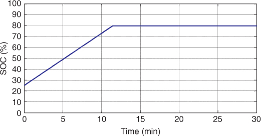
Figure 8.11 Battery SOC changing curve at 3C rate rapid charging.

8.3 Impacts of plug-in charging on electricity network

If a PHEV/BEV is driven 40 miles a day and seven days a week, approximately 3000 kWh of electric energy is consumed by plug-in charging outlets per year. Based on a report by the DOE (U.S. Department of Energy), average monthly residential electricity consumption was 936 kWh and average price was 9.65 cents/kWh in 2007 (DOE report, 2010). The amount would increase by at least 20% if a PHEV/BEV is plugged in per household for charging once a day, which will have a big impact on the existing power distribution systems and electric grid. Such an emerging demand spike to the electric grid, from individual households, has not occurred since air conditioners became widely used in residences in the 1950s (Hadley and Tsvetkova, 2008; Meliopoulos et al. 2009).

8.3.1 Impact on Distribution System

On the distribution system aspect, the plug-in charging of PHEVs/BEVs will affect the size of the feeder, branch circuits, panel board, switches, protective devices, transformers, and so on. The following analysis briefly shows how the changes in household load and load pattern caused by plug-in charging affect the electric power distribution system. Figure 8.12 shows five household daily winter and summer power usage profiles of residential consumers based on the regional average daily winter and summer power usage measured in the field. If we assume that there are two PHEVs in five households and plug-in charging starts at 17:45 and 0:00 with AC-120 and AC-240, respectively, the daily load demand curves with charging two PHEVs are shown in Figs. 8.13, 8.14, 8.15, and 8.16. These figures illustrate that PHEVs/BEVs have a significant effect on power demand; however, the proper setting of charging time could effectively reduce the impact. For example, the peak load will increase to 11 kW from 8.15 kW in summer if we start to charge PHEVs/BEVs at 17:45 by an AC-120 charger, while it will increase to 9 kW from 6 kW if the PHEVs/BEVs are charged from midnight.

Figure 8.12 Average daily load profiles of five households in summer and winter.

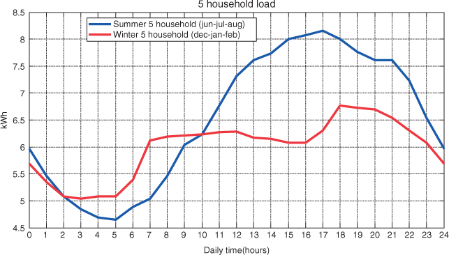
Figure 8.13 Average daily load of five households plus charging two PHEVs by AC-120 charger started at 17:45 in summer and winter.

Figure 8.14 Average daily load of five households plus charging two PHEVs by AC-120 charger started at 00:00 in summer and winter.

Figure 8.15 Average daily load of five households plus charging two PHEVs by AC-240 charger started at 17:45 in summer and winter.

Figure 8.16 Average load of five households plus charging two PHEVs by AC-240 charger started at 00:00 in summer and winter.

8.3.2 Impact on Electric Grid

Electric grids, also known as power grids, interconnect electricity generation stations throughout regions or countries, which allows electricity generated in one region to be sent to users in a different region. They also provide electricity generated by remote power stations for cities and towns in case their local power generators fail or are destroyed by an accident or sabotage. In the interconnection, every generator or synchronous machine connected to the grid operates in synchronism with every other generator, that is, each generator operates at the same speed or frequency while a delicate balance between the input mechanical power and output electric power is maintained. The electrical speed or frequency chosen for this operation is 60 cycles/s, commonly referred to as 60 H/z in North America. Whenever generation is less than actual customer load, the system frequency decreases. On the other hand, when generation exceeds load, the system frequency increases.

For a more detailed explanation, an electric generator is a device that converts mechanical energy to electric energy based on Faraday's electromagnetic principle, called Faraday's law. The device providing the mechanical energy for each generator is called a turbine and is powered either by steam generated by burning fossil fuel or heat derived from nuclear fission or by the kinetic energy from water or wind. The generators are connected with each other and with loads through high-voltage transmission lines, also called power transmission lines. The electricity in the transmission line is stepped down from a high voltage to 120/240 voltage for home or office use.

An important feature of the electric power system is that electricity has to be generated when it is needed because it cannot be efficiently stored. Hence, it is necessary for the generation to be scheduled for every hour in a day to match the loads needed by a sophisticated load forecasting procedure. In addition, some generators are also placed on active standby to provide electricity in case of emergency. Since power grids interconnect so many generators and loads, they routinely undergo a variety of disturbances, and even the act of switching on or off the range in a kitchen can be regarded as a small disturbances. Each power system has a stability margin for it to tolerate a certain level of disturbance. If high or unbalanced demands suddenly present on the power grid, the stability may not be kept. In some cases, the disturbance can cause power outage in a grid section or even ripple through the whole grid, resulting in generators shutting down one after another. The stability of the power grid will be in jeopardy once additional high demands are added in the periods of high demand, for example, on a summer evening, when grids in the whole region are under stress and there is very limited spare power.

With a number of PHEV/BEV added to grids, the overall power demand and demand pattern will change. It could significantly impact the electric grids depending on the time that the battery systems are charged through wall outlets. The common method of handling the changes of power demand and load pattern is to add new electric capacity and reschedule generator operating time; otherwise the reserve margins could be reduced if the electric capacity of the grid does not keep up with the added demand or the change in demand pattern. Depending on the power level, time, and duration of PHEVs/BEVs connected to the grid, it could have various impacts on power grids. Therefore, it is important to explore and understand the consequence of a number of PHEV/BEV connecting to the grid, and the impact analysis should focus on the changes of power demand and pattern from the PHEVs/BEVs. It is also important to analyze and compute real and reactive power flow on each branch and the impact on each component.

8.4 optimal plug-in charging strategy

As discussed above, not only should plug-in chargers be designed as efficient and cost effective is possible and off-peak grid demand be considered but also the grid characteristics should be taken into account. The charging strategies applied to PHEVs/BEVs are as follows:

8.4.1 Optimal Plug-In Charge-Back Point Determination

As discussed in Chapter 5, each type of battery has the best SOC setpoint which enables the battery to have the longest lifetime. For example, the best setpoint of NiMH batteries is around 60% SOC, while it is about 50% SOC for Li-ion batteries. A PHEV/BEV generally has a range of 20–50 miles; however, no matter how many miles the vehicle actually drives, the battery system is normally fully charged or to the designed SOC level when the vehicle is back in the garage.

The optimal PHEV plug-in charge-back point determination method illustrated in this section is based on a PHEV that has 40 electric miles with a 45-Ah Li-ion battery system, and the curve of battery SOC usage versus electric mileage is shown in Fig. 8.17. The corresponding SOC end point after each drive cycle and the designed charge-back point are shown in Fig. 8.18. According to the mechanism of battery life degradation, the best operating setpoint for the battery life is 50% SOC; hence, the optimal plug-in charge-back point should be set as Fig. 8.19 for the given driven mile of the vehicle. The optimal plug-in charge-back point determination algorithm for a PHEV is shown in Fig. 8.20.

Figure 8.17 SOC usage versus electric milage of PHEV.

Figure 8.18 Actual operating SOC setpoint, end point, and charge-back point.

Figure 8.19 Optimal operating SOC setpoint, end point, and charge-back point.

Figure 8.20 Schematic of optimal plug-in charge end-point determination algorithm for PHEVs.

8.4.2 Cost-Based Optimal Plug-In Charging Strategy

The primary goal in developing a plug-in charging algorithm is to obtain the lowest cost for PHEV/BEV owners to charge the battery system back to the desired energy level, while the utility company will set the electric price based on the power demand and electric power availability. Hence, the objective of the plug-in charging strategy is to determine the best charging power and time subject to the constraints of the charger and battery system, required energy (target SOC), and charging time frame. This section presents a cost function–based optimal plug-in charging algorithm, with the flowchart shown in Fig. 8.21.

Figure 8.21 Optimal plug-in algorithm.

Cost Function The cost function for optimizing charging cost can be defined as

8.3

where Cost_energy is the total charging cost, Price(t) is the price of the electric energy at different time periods ($/kWh), t_i is the desired time to start the charge, and t_f is the desired time to complete the charging.

The discrete form is

8.4

where ΔT is the control time interval and N is the number of intervals, N = (t_f − t_i)/ΔT.

Operating Constraint To optimally charge a battery, it is necessary to consider the timing requirement and physical limitations of the charger, battery system, and power outlet. These considerations can be defined as constraints when performing optimization:

• Meet Energy Requirement The total charged energy should be equal to the required energy:

  8.5

  where Energy_chg is the total charged energy in kilowatt-hours, is the energy required to charge the battery from the initial SOC_init to the desired SOC_target target, η_bat and η_charger are the efficiencies of the battery system and the charger, respectively, η_bat is a function of temperature and battery SOC, that is, η_bat = f(SOC, T), and Power(t) = V(t) · I(t) is the charging power between complete time t_f and start time t_i.

• Maximum Allowable Charging Time The maximum charging time period is the time frame in which the battery has to be charged to the target level:

  8.6

  where T_max is the maximum charging time frame and is equal to the difference between set final time t_f and start time t_i.

• Maximum Charging Power The maximum allowable charging power from the charger and battery system is a function of temperature T, battery SOC, and the power limitation of the plug-in charger and the electrical branch circuit:

  8.7

  where Power_max is the maximum allowable charging power in the desired charging period, max(Pwr_{bat(SOC, T)}) is the maximum power that the battery can be charged at the given SOC and temperature, max(Pwr_chg) is the maximum power that the plug-in charger can deliver, and max(Pwr_branch) is the maximum power capacity of the household power outlet.

Optimization Problem The objective of optimization is to find the lowest charging cost, and the problem can be mathematically stated as

8.8

where Cost_energy is the total charging cost, Price(i) is the price of the electric energy at different time periods ($/kW), ΔT is the control time interval, N is the number of intervals, N = (t_f − t_i)/ΔT, t_i is the desired start time to charge, and t_f is the desired complete time of the charging.

Subject to:

8.9

that is,

8.10

Satisfy the constraints:

8.11

where max(Pwr_{bat(SOC, T)}(i)) is the maximum power that the battery can be charged during the ith charging period, max(Pwr_chg(i)) is the maximum power that the plug-in charger can deliver during the ith charging period, and max(Pwr_branch(i)) is the maximum power capacity of the household power outlet during the ith charging period.

Procedures Determining Optimal Charging Schedule Once Price(i) is obtained at each period of time, the optimal charging schedule is determined by the dynamic programming method. As described in Appendix B, the dynamic programming method was developed by Richard Bellman in the early 1950s and is a mathematical method well suited for the optimization of multistage decision problems (Bellman, 1957). Application of the dynamic programming method to solve this problem is shown in Fig. 8.22. At each time point, the costs to charge the battery, as well as the temperature and SOC of the battery, will be computed using the different charging power levels. For example, the SOC and temperature values of the battery system shown in Table 8.1 are calculated during the ith charging period. These values can be used to determine charger and battery efficiency and optimal charging power.

Figure 8.22 Process of optimizing operating points by dynamic programming method.

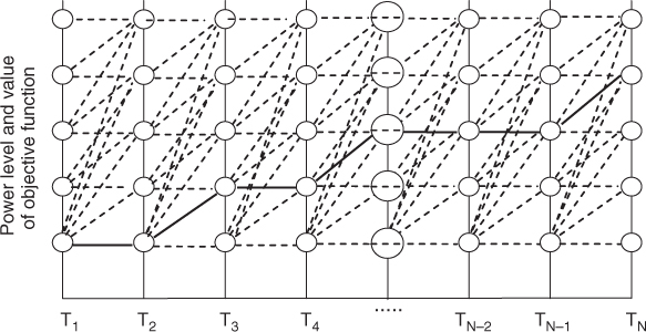
Table 8.1 Example of Calculated Battery SOC and Temperature Corresponding with Different Charging Power During ith Charging Period

Example of Optimal Charging Schedule The parameters of the battery system, plug-in charger, and electric grid are as follows:

• Charger: AC120 charger with 1.5 kW maximum charging capability
• Household electrical branch: with 15 A AC and 1.65 kW maximum power capability
• Battery system: 16-kWh Li-ion battery pack with 45Ah capacity and 360 V nominal voltage
• Charging start time t_i: 18:00 pm
• Charging end time t_f: 6:00 am
• Battery initial SOC_init: 30%
• Target (end) battery SOC_end: 80%
• Calculation time interval: 1800 s (30 min)
• Charging efficiencies of charger and battery system: shown in Tables 8.2 and 8.3
• Electric usage price: shown in Table 8.4

Table 8.2 Operation Efficiency of Plug-in Charger

Table 8.3 Charging Efficiency of Battery System

Table 8.4 Price of Electric Energy

The results show that the optimized charge cost is $0.56, while the uncontrolled charge cost is $1.25 if the charging starts at 18:00 pm, both using smart grid prices. Compared with an uncontrolled plug-in charging schedule, the optimized charging schedule can save the owner over 50% if the charger is connected with the smart grid. The optimized charging schedule is shown in Table 8.5 and the decision-making process is shown in Fig. 8.23.

Figure 8.23 Diagram illustrating determination of plug-in charging power by dynamic programming method.

Table 8.5 Calculated Charging Schedule

References

Bellman, R. E. Dynamic Programming. Princeton University Press, Princeton, NJ, 1957.

U.S. Department of Energy (DOE). “Electric Power Monthly January 2010 With Data for October 2009.” Report No. DOE/EIA-0226 (2010/01), U.S. Energy Information Administration, Office of Coal, Nuclear, Electric and Alternate Fuels, U.S. Department of Energy, 2010.

Hadley, W. S., and Tsvetkova, A. “Potential Impacts of Plug-in Hybrid Electric Vehicles on Regional Power Generation.” Report of Oak Ridge National Laboratory, Oak Ridge, TN, 2008.

Meliopoulos, S., et al. “Power System Level Impacts of Plug-In Hybrid Vehicles.” Final Project Report, Power Systems Engineering Research Center, Georgia Institute of Technology and University of Illinois at Urbana-Champaign, 2009.