
Chapter 6: Energy Management Strategies of Hybrid Vehicle
6.1 Introduction
As stated in previous chapters, hybrid electric vehicles, using a combination of an ICE and electric motor(s), have become a viable alternative to conventional ICE-based vehicles (Powers and Nicastri, 1999). The overall performance of an HEV with respect to fuel economy and emissions reduction depends on the efficiency of the individual components and good coordination of these components. In other words, the energy management strategy (also called power control strategy) in an HEV plays a very important role in the improvement of the fuel economy and reduction of emissions.
Although there are a variety of HEV configurations, achieving maximum fuel economy, minimum emissions, and lowest system cost are the key goals of HEV energy management strategies. In addition, the following problems are often taken into account in the development of HEV energy management strategies:
- Optimize engine operation points/region—The operation points of the engine are set on the optimal points of the torque–speed plane based on the engine mapping data of fuel economy and emissions, as well as compromising between fuel economy and emissions.
- Minimize engine dynamics—The operating speed of an engine is regulated in such a way that any fast fluctuations are avoided, hence minimizing the engine dynamics.
- Minimize engine idle time—The engine's idle time needs to be minimized in order to improve fuel economy and decrease emissions.
- Optimize engine on–off times—The engine on and off times are optimized based on drivers' habits, road and weather conditions, and traffic situations by taking the advantages of dual power sources of HEVs.
- Maximally capture regenerative energy—Optimally set SOC of the battery system in order to maximally capture free regenerative energy based on the drivers' habits and road and weather conditions as well as traffic situations.
- Optimize SOC operating window of the battery system—SOC operating window and swing rates are optimized in order to compromise the battery's life and fuel economy of an HEV.
- Optimize operating points/region of electric motor set—The motor set has a preferred operating region on the torque–speed plane, in which the overall efficiency of the system remains optimum.
- Follow zero-emission policy—In certain areas such as tunnels or workshops, an HEV may need to operate in the pure electric mode. The driving mode of some HEVs should be controlled manually and/or automatically.
The most important and challenging task of the energy management strategy is to distribute the vehicle demand power to the ICE and electric motor optimally and in real time (Rahman et al. 1999). To achieve this, various attempts have been made to develop optimal energy management strategies. For example, Johnson et al. (2000) (presented a control strategy which optimizes vehicle dynamic operating conditions in real time to improve both fuel economy and emissions, Kheir et al. developed fuzzy logic–based energy management strategies for parallel HEVs (Schouten et al. 2003; Kheir et al. 2004), and Sciarretta et al. (2004) proposed a cost–function-based real-time energy management strategy.
We discuss several practical and advanced energy management strategies of an HEV in this chapter. Section 6.2 describes a general rule-based energy management strategy. Section 6.3 presents the implementation of a fuzzy logic–based HEV energy management strategy. A dynamic programming approach and implementation are proposed in Section 6.4. Optimization results and comparisons are given in Section 6.5.
6.2 Rule-based energy management strategy
A rule-based energy management strategy is the one most commonly used in light to medium-size HEVs, especially in the early development stage. The fundamental rules of this type energy management strategy include:
An example of power split results from the rule-based energy management strategy to a parallel HEV is shown in Fig. 6.1. From the strategy, if the vehicle demand power is less than 8 kW, only the electric motor is used to drive the vehicle; if the vehicle demand power is between 8 and 40 kW, the ICE mainly powers the vehicle, and whether the battery is charged or not depends on the other inputs, such as the SOC of the ESS; if the vehicle demand power is between 40 and 70 kW, the ICE outputs a constant 40 kW power, and the electric motor generates additional mechanical power to meet the drivability requirement; and if the vehicle demand power is between 70 and 90 kW, the electric motor outputs its maximum of 30 kW power and the ICE outputs additional power to meet the power requirement of the vehicle.
Figure 6.1 Vehicle demand power split based on rule-based energy management strategy.

6.3 Fuzzy logic–based energy management strategy
Due to the complexity of a hybrid vehicle system, conventional design methods that rely on an exact mathematical model are limited. Fuzzy control is one of the most active and fruitful areas where fuzzy set theory is applied. It is feasible and advantageous to employ fuzzy logic control techniques to design the energy management strategy for a hybrid vehicle system. In this section, a fuzzy logic control method is briefly introduced, and then a fuzzy logic–based energy management strategy is presented, including a detailed design example and design procedures.
6.3.1 Fuzzy Logic Control
Fuzzy logic control theory mainly includes fuzzy set theory and fuzzy logic. Fuzzy set theory is an extension of conventional set theory, and fuzzy logic is an extension of conventional logic (Tanaka, 1996). Some basic concepts of fuzzy sets and logic are introduced below.
A. Fuzzy Sets and Membership Functions Fuzzy sets were proposed to deal with vague words and expressions. Lotfi A. Zadeh (1965) first introduced the concept of fuzzy sets, whose elements have degrees of membership. In mathematics, a fuzzy set A on the universe X is a set defined by a membership function μA representing a mapping
where the value of μA(x) in the fuzzy set A is called the membership value, which represents the degree of x belonging to the fuzzy set A. The membership value indicated by equation 6.1 can be an arbitrary real value between 0 and 1. The closer the value of μA is to 1, the higher the grade of membership of the element x in fuzzy set A. For example, if μA = 1, the element x completely belongs to the fuzzy set A, while if μA = 0, the element x does not belong to the fuzzy set A. To illustrate the features of fuzzy sets, the following examples are given based on the speed of a vehicle and compared with conventional sets which are exactly defined and called “crisp sets.”
Suppose that three vehicle speeds A, B, and C are given as
![]()
Comparing the vehicle speeds defined in Fig. 6.2 and Fig. 6.3, we get values of the characteristic function in crisp sets and membership function in fuzzy sets in Table 6.1. The values of the characteristic function in the conventional set indicate that A belongs to the low set, B belongs to the medium set, and C belongs to high set. The values of the membership function in the fuzzy set indicate that A belongs to the low set in the grade of 8/9 and to the medium set in the grade of 1/9, and A does not belong to the high set; B belongs to the low set in the grade of 1/3 and to the medium set in the grade of 2/3; and C belongs to the medium set in the grade of 2/3 and to the high set in the grade of 1/3. In reality, if we are to express these speeds linguistically, the expression may be
![]()
Figure 6.2 Crisp set of vehicle.

Figure 6.3 Fuzzy set of vehicle.
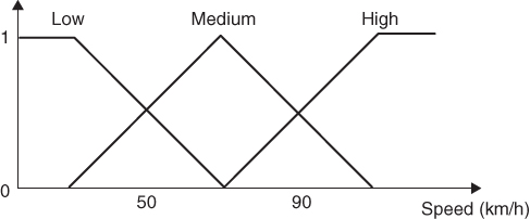
Table 6.1 Value of Characteristic Function in Crisp Sets and Membership Function in Fuzzy Sets
 |
B. Mathematical Expression of Fuzzy Sets and Membership Functions The detailed values of a membership function in the defined fuzzy set can be calculated based on the following definition:
The symbol “/” in equation 6.2 is called a separator. An element of the universe is written on the right of the separator and the membership value of the fuzzy set A is written on the left.
Figure 6.4 Triangular fuzzy set expression.

Figure 6.5 Trapezoidal fuzzy set expression.

C. Properties, Equality, and Inclusion of Fuzzy Sets If we assume that A, B, and C are fuzzy sets on the universe X, they have the following properties:
- Idempotent law:

- Communicative law:

- Associative law:

- Distributive law:

- Double-negation law:

- De Morgan's law:

- Equality:

- Inclusion:

D. Fuzzy Relations A fuzzy relation is an extension of relations in conventional set theory. In addition to being applied in practical engineering systems, fuzzy relations are also widely applied in psychology, medicine, economics, and sociology. A definition of an n-ary fuzzy relation is given by Kazuo Tanaka (1996) as follows:
6.3 ![]()
where μR is the membership function of R given as
6.4 ![]()
In practice, the most used fuzzy relation is the binary fuzzy relation and is expressed as follows: If given the universe X and Y,
6.5 ![]()
the binary fuzzy relation of X and Y is expressed as
6.6

In this fuzzy relation, “similar,” the degree of resemblance between son x1 and father y1 is 0.8; the degree of resemblance between son x1 and mother y2 is 0.3; the degree of resemblance between daughter x2 and father y1 is 0.3; and the degree of resemblance between daughter x2 and mother y2 is 0.6. This relation indicates that the daughter is more similar to the mother than the son, but the son is much more similar to the father than the daughter.
E. Fuzzy Reasoning Inference rules of fuzzy reasoning are expressed in IF–THEN format, which are called fuzzy IF–THEN rules. The fuzzy reasoning methods can be classified as direct and indirect methods. The most popular reasoning methods are direct methods which include the Mamdani method, the Takagi–Sugeno method, and other simplified methods (Mamdani, 1974; Takagi and Sugeno, 1985). Direct fuzzy reasoning methods use the inference rule format
where A, B, and C are fuzzy set. In the IF–THEN rule, the term following IF is called the premise, and the term following THEN is called the consequence. Therefore, variables x and y are premise variables and the variable z is the consequence variable.
-
Rule 1:IF the distance between cars is shortAND the vehicle speed is lowTHEN maintain the speed (hold the current acceleration pedal position)
-
Rule 2:IF the distance between cars is short and two cars are closingAND the vehicle speed is highTHEN reduce the speed (step on the brake pedal)
-
Rule 3:IF the distance between cars is longAND the vehicle speed is lowTHEN increase the speed (step on the acceleration pedal)
-
Rule 4:IF the distance between cars is longAND the vehicle speed is highTHEN maintain the speed (hold the current acceleration pedal position)
F. Conversion of IF–THEN Rules to Fuzzy Relations Let us consider a fuzzy reasoning with two positions in equation (6.7). It can be simplified as
It should be noted that equation 6.8 cannot be described by the preceding relation ![]() as A and B are subsets of different sets X and Y. Zadeh (1965) and Mamdani (1974) gave the following conversion formulas:
as A and B are subsets of different sets X and Y. Zadeh (1965) and Mamdani (1974) gave the following conversion formulas:
- Zadeh's formula:
6.9

- Mamdani's formula:
6.10

where μR(x, y, z), μA(x), μB(y), μc(z) are membership values.
- Rule 1:

- Rule 2:

where X = {x1x2x3} and A1, A2 ⊂ X, Y = {y1y2y3} and B1, B2 ⊂ Y, Z = {z1z2z3} and C1, C2 ⊂ Z; the fuzzy sets A1, A2, B1, B2, C1, C2 are given as


6.3.2 Fuzzy Logic–Based HEV Energy Management Strategy
In the recent development of hybrid vehicle systems, fuzzy logic has been used to control the energy flow of an HEV based on the following principles:
- A vehicle's required power has to be met at all times during operation.
- A driver's inputs from brake and acceleration pedals are satisfied consistently.
- The SOC of the battery system is maintained in a certain window at all time.
- The overall system efficiency is maximized during operation.
A fuzzy logic–based HEV energy management strategy can be designed from the following procedures:
A. Establish Fuzzy Rules Based on the configuration of an HEV and engineering design objectives, establish fuzzy rules as shown in Table 6.2, where ωveh is the vehicle speed, Pveh is the vehicle demand power, Pmot is the required power from the electric motor (positive is power, negative is regenerative), SOCmin is the allowable minimum SOC of the battery system, and SOCmax is the allowable maximum SOC of the battery system.
Table 6.2 Fuzzy Logic Rules of Energy Management Strategy of HEV
| No. | Rule |
| 1 | If SOC ≥ SOCmax, ωveh = low, and Pveh = negative high, then Pmot = zero |
| 2 | If SOC ≥ SOCmax, ωveh = low, and Pveh = negative low, then Pmot = zero |
| 3 | If SOC ≥ SOCmax, ωveh = low, and Pveh = zero, then Pmot = zero |
| 4 | If SOC ≥ SOCmax, ωveh = low, and Pveh = positive low, then Pmot = positive low |
| 5 | If SOC ≥ SOCmax, ωveh = low, and Pveh = positive high, then Pmot = positive high |
| 6 | If SOC ≥ SOCmax, ωveh = medium, and Pveh = negative high, then Pmot = zero |
| 7 | If SOC ≥ SOCmax, ωveh = medium, and Pveh = negative low, then Pmot = zero |
| 8 | If SOC ≥ SOCmax, ωveh = medium, and Pveh = zero, then Pmot = zero |
| 9 | If SOC ≥ SOCmax, ωveh = medium, and Pveh = positive low, then Pmot = positive low |
| 10 | If SOC ≥ SOCmax, ωveh = medium, and Pveh = positive high, then Pmot = positive high |
| 11 | If SOC ≥ SOCmax, ωveh = high, and Pveh = negative high, then Pmot = zero |
| 12 | If SOC ≥ SOCmax, ωveh = high, and Pveh = negative low, then Pmot = zero |
| 13 | If SOC ≥ SOCmax, ωveh = high, and Pveh = zero, then Pmot = zero |
| 14 | If SOC ≥ SOCmax, ωveh = high, and Pveh = positive low, then Pmot = positive low |
| 15 | If SOC ≥ SOCmax, ωveh = high, and Pveh = positive high, then Pmot = positive high |
| 16 | If SOCmin ≤ SOC ≤ SOCmax, ωveh = low, and Pveh = negative high, then Pmot = negative high |
| 17 | If SOCmin ≤ SOC ≤ SOCmax, ωveh = low, and Pveh = negative low, then Pmot = negative low |
| 18 | If SOCmin ≤ SOC ≤ SOCmax, ωveh = low, and Pveh = zero, then Pmot = zero |
| 19 | If SOCmin ≤ SOC ≤ SOCmax, ωveh = low, and Pveh = positive low, then Pmot = positive low |
| 20 | If SOCmin ≤ SOC ≤ SOCmax, ωveh = low, and Pveh = positive high, then Pmot = positive high |
| 21 | If SOCmin ≤ SOC ≤ SOCmax, ωveh = medium, and Pveh = negative high, then Pmot = negative high |
| 22 | If SOCmin ≤ SOC ≤ SOCmax, ωveh = medium, and Pveh = negative low, then Pmot = negative low |
| 23 | If SOCmin ≤ SOC ≤ SOCmax, ωveh = medium, and Pveh = zero, then Pmot = zero |
| 24 | If SOCmin ≤ SOC ≤ SOCmax, ωveh = medium, and Pveh = positive low, then Pmot = positive low |
| 25 | If SOCmin ≤ SOC ≤ SOCmax, ωveh = medium, and Pveh = positive high, then Pmot = positive low |
| 26 | If SOCmin ≤ SOC ≤ SOCmax, ωveh = high, and Pveh = negative high, then Pmot = negative high |
| 27 | If SOCmin ≤ SOC ≤ SOCmax, ωveh = high, and Pveh = negative low, then Pmot = negative low |
| 28 | If SOCmin ≤ SOC ≤ SOCmax, ωveh = high, and Pveh = zero, then Pmot = zero |
| 29 | If SOCmin ≤ SOC ≤ SOCmax, ωveh = high, and Pveh = positive low, then Pmot = positive low |
| 30 | If SOCmin ≤ SOC ≤ SOCmax, ωveh = high, and Pveh = positive high, then Pmot = zero |
| 31 | If SOC ≤ SOCmin, ωveh = low, and Pveh = negative high, then Pmot = negative high |
| 32 | If SOC ≤ SOCmin, ωveh = low, and Pveh = negative low, then Pmot = negative low |
| 33 | If SOC ≤ SOCmin, ωveh = low, and Pveh = zero, then Pmot = negative low |
| 34 | If SOC ≤ SOCmin, ωveh = low, and Pveh = positive low, then Pmot = negative low |
| 35 | If SOC ≤ SOCmin, ωveh = low, and Pveh = positive high, then Pmot = zero |
| 36 | If SOC ≤ SOCmin, ωveh = medium, and Pveh = negative high, then Pmot = negative low |
| 37 | If SOC ≤ SOCmin, ωveh = medium, and Pveh = negative low, then Pmot = negative low |
| 38 | If SOC ≤ SOCmin, ωveh = medium, and Pveh = zero, then Pmot = negative low |
| 39 | If SOC ≤ SOCmin, ωveh = medium, and Pveh = positive low, then Pmot = negative low |
| 40 | If SOC ≤ SOCmin, ωveh = medium, and Pveh = positive high, then Pmot = zero |
| 41 | If SOC ≤ SOCmin, ωveh = high, and Pveh = negative high, then Pmot = negative high |
| 42 | If SOC ≤ SOCmin, ωveh = high, and Pveh = negative low, then Pmot = negative low |
| 43 | If SOC ≤ SOCmin, ωveh = high, and Pveh = zero, then Pmot = negative low |
| 44 | If SOC ≤ SOCmin, ωveh = high, and Pveh = positive low, then Pmot = negative low |
| 45 | If SOC ≤ SOCmin, ωveh = high, and Pveh = positive high, then Pmot = zero |
B. Formulize Fuzzy Relations from Fuzzy IF–THEN Rules Based on the configuration and specification of the hybrid vehicle system, if the fuzzy sets are defined by equations 6.11–6.14, the fuzzy IF–THEN rules in Table 6.2 can be written as in Table 6.3.
6.12 ![]()
6.13 ![]()
Table 6.3 Formulized Fuzzy Logic Rules
| No. | Rule |
| 1 | If x is A3, y is B1, and z is C1, then s is D3 |
| 2 | If x is A3, y is B1, and z is C2, then s is D3 |
| 3 | If x is A3, y is B1, and z is C3, then s is D3 |
| 4 | If x is A3, y is B1, and z is C4, then s is D4 |
| 5 | If x is A3, y is B1, and z is C5, then s is D5 |
| 6 | If x is A3, y is B2, and z is C1, then s is D3 |
| 7 | If x is A3, y is B2, and z is C2, then s is D3 |
| 8 | If x is A3, y is B2, and z is C3, then s is D3 |
| 9 | If x is A3, y is B2, and z is C4, then s is D4 |
| 10 | If x is A3, y is B2, and z is C5, then s is D5 |
| 11 | If x is A3, y is B3, and z is C1, then s is D3 |
| 12 | If x is A3, y is B3, and z is C2, then s is D3 |
| 13 | If x is A3, y is B3, and z is C3, then s is D3 |
| 14 | If x is A3, y is B3, and z is C4, then s is D4 |
| 15 | If x is A3, y is B3, and z is C5, then s is D5 |
| 16 | If x is A2, y is B1, and z is C1, then s is D1 |
| 17 | If x is A2, y is B1, and z is C2, then s is D2 |
| 18 | If x is A2, y is B1, and z is C3, then s is D3 |
| 19 | If x is A2, y is B1, and z is C4, then s is D4 |
| 20 | If x is A2, y is B1, and z is C5, then y is D5 |
| 21 | If x is A2, y is B2, and z is C1, then s is D1 |
| 22 | If x is A2, y is B2, and z is C2, then s is D2 |
| 23 | If x is A2, y is B2, and z is C3, then s is D3 |
| 24 | If x is A2, y is B2, and z is C4, then s is D4 |
| 25 | If x is A2, y is B2, and z is C5, then s is D4 |
| 26 | If x is A2, y is B3, and z is C1, then s is D1 |
| 27 | If x is A2, y is B3, and z is C2, then s is D2 |
| 28 | If x is A2, y is B3, and z is C3, then s is D3 |
| 29 | If x is A2, y is B3, and z is C4, then s is D4 |
| 30 | If x is A2, y is B3, and z is C5, then s is D5 |
| 31 | If x is A1, y is B1, and z is C1, then s is D1 |
| 32 | If x is A1, y is B1, and z is C2, then s is D2 |
| 33 | If x is A1, y is B1, and z is C3, then s is D2 |
| 34 | If x is A1, y is B1, and z is C4, then s is D2 |
| 35 | If x is A1, y is B1, and z is C5, then s is D3 |
| 36 | If x is A1, y is B2, and z is C1, then s is D1 |
| 37 | If x is A1, y is B2, and z is C2, then s is D2 |
| 38 | If x is A1, y is B2, and z is C3, then s is D2 |
| 39 | If x is A1, y is B2, and z is C4, then s is D2 |
| 40 | If x is A1, y is B2, and z is C5, then s is D3 |
| 41 | If x is A1, y is B3, and z is C1, then s is D1 |
| 42 | If x is A1, y is B3, and z is C2, then s is D2 |
| 43 | If x is A1, y is B3, and z is C3, then s is D2 |
| 44 | If x is A1, y is B3, and z is C4, then s is D2 |
| 45 | If x is A1, y is B3, and z is C5, then s is D3 |
The following fuzzy sets are defined and shown in Fig. 6.6:

Figure 6.6 Fuzzy sets for HEV energy management.

Mamdani's conversion method can be further used to establish fuzzy relations from the fuzzy IF–THEN rules described above. Because there are four elements, x, y, z, and s, the conversion formula is
6.15 ![]()
where x is SOC, y is vehicle speed (km/h), zis vehicle demand power (kW), and s is the determined motor power (positive is propulsion power, negative is regenerative brake power), i, j = 1, 2, 3, k, m = 1, 2, 3, 4, 5.
Since the given fuzzy relation is four dimensional, the rules contain three propositions in the premises. The three elements of the fuzzy array are calculated by Mamdani's formula as
6.16 ![]()
6.17 ![]()
6.18 ![]()


By the conversion formula (6.15), the fuzzy relations from R1 to R45 can be obtained as follows.


The overall fuzzy relation R is given by
6.19 


C. Reasoning by Fuzzy Relations After fuzzy IF–THEN rules and fuzzy relations are established, the next step is to reason the control output using fuzzy relations, that is, to command electric motor and ICE power to meet the vehicle demand power. In the example given above, there are three inputs x, y, z and one output s. For the input of fuzzy set A on X, fuzzy set B on Y, and fuzzy set C on Z, the output fuzzy set D on S can be obtained as
where ° represents composition.
When there are three variables in the premise, fuzzy relation R has four terms (relation between x, y, z, and s). In the above example, a three-stage composition process for reasoning is employed as equation 6.20.
-
Battery SOC = 56% (minimum SOCmin = 40%, maximum SOCmax = 60%)
- Vehicle speed = 30 km/h
- Vehicle demand power = 25 kW
Determine the required power from the electric motor and ICE based on the fuzzy rules of the energy management introduced above.


Through defuzzification, the definite value of the required power from the electric motor is 18.626 kW; therefore the required power from the ICE should be equal to 25 − 18.626 = 6.374 kW to meet the drivability requirement of the vehicle.
D. Diagram of Fuzzy Logic–Based HEV Energy Management Strategy The overall fuzzy logic–based energy management strategy diagram is shown in Fig. 6.7. This strategy first employs fuzzy logic methodology to calculate the required power from the motor based on the vehicle speed and demand power as well as the SOC of the battery system, then feeds the calculated power to the final decision block to decide how much power the electric motor should generate and how much the ICE should output to meet the vehicle power requirement. The final decision is to adjust the motor power calculated by fuzzy logic to make the ICE work at the predetermined operating points. For example, in the circumstance described in Example 6.7, the motor power (18.626 kW) calculated by fuzzy logic is adjusted to 18 kW and has ICE output of 7 kW to meet the 25 kW power requirement of the vehicle.
Figure 6.7 Fuzzy logic–based HEV energy management strategy.

6.4 Determination of optimal ICE operating points of hybrid vehicle
Since the ICE working state directly affects the fuel economy and emissions of an HEV, it is necessary to determine the optimum operating points based on the hybrid vehicle driving characteristics. This section introduces a two-step optimization method determining the optimal operating points for an HEV based on engine mapping data and the power requirements of practical drive cycles.
6.4.1 Mathematical Description of Problem
Selecting the operating points (OPs) for the ICE in an HEV is an important calibration task. Conventionally, they are determined by experienced engineers from torque–speed or power–speed mapping data. Fundamentally, determining OPs is a trade-off between emissions and fuel consumption rate, and the optimum problem can be formalized as follows: Find the optimal OPs of the ICE in an HEV:
6.21 ![]()
Minimize the following two objective functions:
6.22 ![]()
The objective function ![]() , objective function
, objective function ![]() , and constraints are defined as
, and constraints are defined as
where a1, … , a5 are the weight factors corresponding to the relative importance of the fuel economy and emissions, “fuel” is fuel consumption, NOx is nitrogen oxides, CO is carbon monoxide, HC is hydrocarbon, PM is particulate matter, b1, ![]() , bn, are the weight factors corresponding to the frequencies of the power level at which the ICE operates in a practical driving situation of an HEV, JP1 is the value of objective function J1 that the ICE works at zero power output (idle state), and JPn is the value of objective function J1 that the ICE works at the nth power level:
, bn, are the weight factors corresponding to the frequencies of the power level at which the ICE operates in a practical driving situation of an HEV, JP1 is the value of objective function J1 that the ICE works at zero power output (idle state), and JPn is the value of objective function J1 that the ICE works at the nth power level:
where OP1, … , OPn are the operating speeds of an ICE corresponding to the required power/torque points, for example, OP1 is the operating speed of the ICE at zero output power (idle state) and OPn is the operating speed when the ICE outputs its maximum power. This constraint means that the higher required power needs higher operating speed.
6.4.2 Procedures Determining Optimal Operating Points
The two-step optimization algorithm shown in Fig. 6.8 can be used to solve the above optimization problem. The strategy first uses the golden section search algorithm to obtain the local optimal operating point at each specific operating power level of the ICE, which minimizes the objective function J1 (6.23) without considering objective function J2 (6.24) and the constraint (6.25); then, dynamic programming is employed to get the global minimum of the optimization problem which minimizes the objective function J2 subject to the practical operating constraints.
Figure 6.8 Algorithm to find optimal points for ICE in HEV.

The procedure is as follows:
6.4.3 Golden Section Search Method
Golden section search is a commonly used method to solve the one-dimensional optimization problem. If the distance between two ends (say, a and c) is L, the optimal middle point b for searching is the fractional distance 0.618 from one end and 0.382 from the other end. As this fraction was called the golden ratio in ancient Greece, the searching method based on this section is named golden section (Rao, 1996). The golden section search process is illustrated in Fig. 6.9. The minimum is bracketed by points 1, *, and 2. Based on the golden section search method, the objective function value is evaluated at point 3, which is the fractional distance 0.382 from point 2 and 0.618 from point 1, and point 2 will be replaced by point 3; then the objective function value is evaluated at point 4, which is the fractional distance 0.382 from point 1 and 0.618 from point 3, and the point 1 will be replaced by point 4; then it is evaluated at 5, which replaces 3. After several steps as shown, the minimum is bracketed in a smaller and smaller range; for example, after three steps, the minimum will be bracketed between points 4 and 5.
Figure 6.9 Golden section search.

6.4.4 Determining Optimal Operating Points
The search process for the operating points of an ICE can be stated as follows: After the local optimization results for the objective function J1 are obtained based on a search method such as golden search and the objective function J2 and the constraint equation are given, the optimal operating points of the ICE of an HEV can be found and they are the points that make the sum of objective function J1 from power level 1 to n be minimum. The mathematical expression is
6.26 
6.27 ![]()
where opi is the ICE operating speed corresponding to the operating power level i, bi is the weight for the given operating power level, and JPi is the value of objective function J1 corresponding to the operating speed at the given operating power level.
It is obvious that the above is a multistage decision problem, which means that the operating speed has to be determined at the given operating power level of the ICE, shown in Fig. 6.10. In other words, the objective function Ji needs to be minimized in order to achieve the optimal fuel economy and emissions. The dynamic programming technique is well suited to solve such problems (Bellman, 1957).
Figure 6.10 Process-optimizing operating points.

6.4.5 Example of Optimal Determination
This example is based on a series HEV with the following system parameters:
- ICE: 50 kW maximum-power diesel engine, speed–torque and speed–power curves shown in Fig. 6.11, and mapped fuel consumption and emission data shown in Table 6.4
Table 6.4 Corresponding Engine Mapping Data for Optimizing Operating Points
 |
- Generator: 45 kW rated maximum power, maximum usable power 40 kW, speed–torque and speed–power curves shown in Fig. 6.12
- Electric motor: 67 kW rated maximum power, speed–torque shown in Fig. 6.13
- Gear reduction ratio: 3.05:1
- DC/DC converter: 1.4 kW
- Battery system: 8.5 Ah NiMH battery with 70% initial SOC
- Final drive ratio: 4.1:1
- Vehicle weight: 2400 kg
- Vehicle Cd = 0.46
- Wheel radius: 0.335 m
- Schedule road grade is 0%
Figure 6.11 Curves of power versus speed (solid line) and torque versus speed (dashed line) of ICE.

Figure 6.12 Curves of torque versus speed (solid line) and power versus speed (dashed line) of generator.

Figure 6.13 Curves of torque versus speed (solid line) and power versus speed (dashed line) of electric motor.

The optimal operating points are determined from the following procedure based on the method introduced in previous sections. For a more detailed description of the optimal ICE operating point determination method, the interested reader can refer to Liu and Bouchon (2008a).
Table 6.5 Values of Objective Function 1 (J1) at Each Power Requirement Point

Figure 6.14 Determined optimal operating points when objective Functions 1 and 2 are set as J1 = 10.0 · fuel + 1.0 · NOx + 1.0 · CO + 1.0 · HC and J2 = 1.0 · JP1 + 1.0JP2 + 1.0JP3 + 5.0JP4 + 10.0JP5 + 5.0JP6 + 1.0JP7 + 1.0JP8.

6.4.6 Performance Evaluation
To illustrate the effect of the optimized operating points, this section presents two performance studies on a parallel HVE based on the EPA75 drive cycle shown in Fig. 6.15. The required ICE power over the cycle, shown in Fig. 6.16, is commanded by the energy management algorithm of the HEV. The manually set ICE operating points are [1600, 1700, 2000, 2200, 2200, 2200, 2400, 2600] RPM corresponding to the operating power levels [0, 5, 10, 15, 20, 25, 30, 35] kW, shown as Fig. 6.17.
Figure 6.15 Federal U.S. urban drive schedule.

Figure 6.16 Required ICE power over EPA75 drive cycle.

Figure 6.17 Manually set operating points.

Comparison Study 1 If the weight factors of the objective function J1 are set as [10.0 1.0 1.0 1.0] shown equation 6.8 and the weight factors of the objective function J2 are set as [1.0 1.0 1.0 5.0 10.0 5.0 1.0 1.0] shown in equation (6.29), the computed optimal operating points are [900, 1500, 1500, 1700, 1800, 1800, 2100, 2600] RPM corresponding to the given operating power level based on the engine mapping data shown in Table 6.4, the curve shown as Fig. 6.18. The objective function J1 minimizes fuel usage over the drive cycle by putting a bigger penalty factor on the fuel usage term; while the objective function J2 is minimizes global fuel consumption over the cycle by putting a bigger penalty factor on the 25-kW power level that at which the ICE mostly operates.
6.28 ![]()
Figure 6.18 Optimized operating point curve by J1 = 10.0 * fuel + 1.0 · NOx + 1.0 · CO + 1.0 · HC and J2 = 1.0JP1 + 1.0JP2 + 1.0JP3 + 5.0JP4 + 10.0JP5 + 5.0JP6 + 1.0JP7 + 1.0JP8.

The achieved average results over the drive cycle are as follows:
The comparison shows that if the ICE operates at the optimal operating points over the EPA 75 cycle, the fuel economy is improved by approximately 16.2%, and CO and HC emissions are reduced by about 45.8 and 25.1%, respectively at the cost of 28.7% increase of NOx emissions. The detailed comparison curves on fuel consumption and emissions are shown in Figs. 6.19, 6.20, 6.21, and 6.22.
Figure 6.19 Fuel consumption versus EPA drive cycle.

Figure 6.20 NOx emission versus EPA drive cycle.

Figure 6.21 CO emission versus EPA drive cycle.
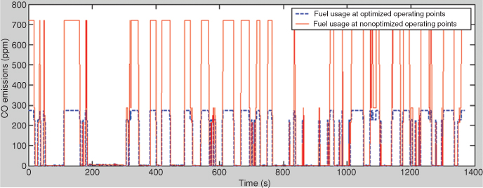
Figure 6.22 HC emission versus EPA drive cycle.

Comparison Study 2 Different from study case 1, if there are bigger penalty factors on the fuel consumption and NOx emission of the objective function J1 and bigger penalty factors on the 20-, 25-, and 30-kW operating power levels of the objective function J2, the optimized operating points are [1700, 1700, 1900, 2300, 2300, 2300, 2400, 2600] RPM, the curve shown in Fig. 6.23. The detailed objective functions are:
6.30 
6.31 
Figure 6.23 Optimized operating points when J1 = 10.0 · fuel + 10.0 · NOx + 1.0 · CO + 1.0 · HC and J2 = 1.0JP1 + 1.0JP2 + 1.0JP3 + 5.0JP4 + 10.0JP5 + 5.0JP6 + 1.0JP7 + 1.0JP8.

The study results show that the average fuel consumption is 2.61 kg/h, the average NOx emissions are 66.24 ppm, the average CO emissions is 103.2 ppm, and the average HC emission is 120.2 ppm when the ICE operates at the optimized operating points by the above objective functions. Compared with the case where the ICE operates at the manually set operating points, the optimal operating points improve the fuel economy by approximately 1.5% and reduce NOx emissions by about 0.6%, which are traded off by increasing CO and HC emissions about 20.8 and 7%, respectively. The detailed comparison curves on fuel consumption and emissions are shown in Figs. 6.24, 6.25, 6.26, and 6.27.
Figure 6.24 Fuel usage comparison versus EPA drive cycle.

Figure 6.25 NOx emission versus EPA drive cycle.

Figure 6.26 CO emission versus EPA drive cycle.

Figure 6.27 HC emission versus EPA drive cycle.

6.5 Cost function–based optimal energy management strategy
Engineering practices have proven that hybrid vehicles can significantly improve fuel economy and reduce greenhouse gas emissions as well as urban air pollutants relative to conventional gasoline or diesel engine vehicles. A crucial and challenging task in hybrid vehicle system design is to optimally distribute the total vehicle required power to the ICE and electric motor. The quality of this decision directly affects the overall performance of a vehicle, including drivability, fuel economy, and emissions. Therefore, most automobile companies, including GM, Toyota, and Ford, developed many new technologies and filed many patents on energy management strategies of hybrid vehicles. Many scientists and engineers have also proposed various approaches to achieve optimal fuel economy and emissions (Powers and Nicastri, 1999; Rahman et al., 1999). These include real-time optimization algorithms for fuel economy and emissions and various intelligent energy management methods and cost function–based strategies (Johnson et al., 2000; Won et al., 2003; Schouten et al., 2003; Piccolo et al., 2001; Fussey et al., 2004; Cox and Bertness, 2005; Liu and Bouchon, 2008b).
This section outlines a cost function–based HEV energy management strategy. A detailed example is given to illustrate how to configure the objective function and adapt the equivalent fuel consumption of the electric motor in real time based on the amount of recovered energy from regenerative braking. This section also presents how to take the constraints of power requirement and battery life into account in a practical hybrid vehicle system design.
6.5.1 Mathematical Description of Cost Function–Based Optimal Energy Management
A. Definition of Cost Function The cost function to optimize the energy flow of a hybrid vehicle can be defined as
6.32 
In equation 6.1, Cfuel is the weight factor for the actual real fuel cost, which can be calibrated based on the fuel consumption map of the engine, such as Table 6.4, in grams per kilowatts power per sampling time of engine control system [g/(kW · Teng)]:
6.33 ![]()
The weight factor Celectric is for electric energy cost, which is normalized and equalized to the fuel cost of the engine. The normalization is based on the best fuel rate of the engine at the current operating speed and efficiencies of the electric motor and battery system as given by
6.34 ![]()
where ηbat is the efficiency of the battery system, where ηbat = ηdischarge if Powermot ≤ 0 and ηbat = ηcharge if Powermot > 0 in cost function (6.32), and ηmot is the efficiency of the motor/inverter system at the current operating condition.
The weight factor ![]() is for the cost of battery life loss, which is a function of the battery's SOC, temperature, and electric power:
is for the cost of battery life loss, which is a function of the battery's SOC, temperature, and electric power:
6.35 ![]()
The weight factor ![]() is for the cost that the SOC of the battery system is away from the desired operating setpoint SOCdesired, which is a function of the battery's SOC, temperature, and electric power:
is for the cost that the SOC of the battery system is away from the desired operating setpoint SOCdesired, which is a function of the battery's SOC, temperature, and electric power:
6.36 ![]()
All cost weight factors in cost function (6.32) are normalized with the real fuel consumption rate of the engine at the given operating condition.
B. Required Power In a parallel hybrid vehicle system, the vehicle required power is always equal to the sum of the engine's output power and motor's output power. The engine always outputs positive power, but the motor's power can be positive (power) or negative (regenerative). Therefore, we have
6.37 ![]()
6.38 ![]()
C. Operating constraints To assign the vehicle demand power to the ICE and electric motor optimally, it is necessary to consider the physical limitations of each component in a practice hybrid vehicle. The limitations can be defined as constrains when performing optimization.
- Constraints from Energy Storage System
(a) Maximum Charging Power The maximum allowable charging power availability of the ESS is a function of temperature, SOC, and state of health (SOH) at the given operating conditions. The following equation can be used to describe this constraint:
6.39
 where
where is the maximum charging power availability of the ESS in the next control period.(b) Maximum Discharging Power The maximum allowable discharging power availability of the ESS is also a function of temperature, SOC, and SOH. The following equation can be used to describe this constraint:
6.40
 where
where is the maximum discharging power availability of the ESS in next control period.
 - Constraints from Electric Motor
(a) Maximum Propulsion Power The maximum propulsion power of the motor is a function of the temperature, speed, and torque of the motor at the given operating condition. The following equation can be used to describe the constraint:
6.41

where
 is the propulsive power constraint of the motor in the next control period.(b) Maximum Regenerative Power
The maximum regenerative power of the motor is also related to the temperature, speed, and torque of the motor at the given operating condition. It can be expressed by the equation
6.42

where
 is the regenerative power constraint of the motor in the next control period.
 - Constraints from Engine
(a) Maximum Propulsion Power The maximum propulsion power of the engine is a function of its speed, which can be described by
6.43

D. Description of Optimization Problem The optimization objective is to find the optimal power distribution to the ICE and electric motor of an HEV so the vehicle has the best fuel economy at the current operating condition. The optimization problem can be stated mathematically as follows:
6.44 ![]()
6.45 ![]()
6.46 ![]()
6.47 ![]()
Note: the sign conventions of motor and battery system are normally opposite in hybrid vehicle system, for example, the “+” is propulsion for motor but is charge for battery in which the motor is in regenerative.
6.5.2 Example of Optimization Implementation
The given optimization example is based on the following hybrid vehicle system configuration, parameters, and operating condition.
- Hybrid vehicle system configuration: parallel
- Control period of time: 10 ms
- ICE: 50 kW maximum power diesel engine, the mapped fuel consumption and emission data are listed in Table 6.4 and modified to milligrams per kilowatt-hour per 10 ms from the original grams per kilowatt-hour
- Electric motor: 30 kW rated maximum power
- The vehicle operating speed: 110 km/h
- The vehicle demanding power: 40 kW
- SOC setpoint of the battery system: 60%
- SOC operation window of the battery system: 40–80%
- Battery age: beginning of life
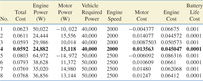
The real-time power split optimization algorithm diagram is shown in Fig. 6.28. The detailed optimization results are listed in Table 6.6. The best power combination at the given operating condition is that the engine outputs 25 kW power and the electric motor outputs 15 kW power.
Figure 6.28 Real-time power split optimization algorithm.

Table 6.6 Evaluated Results in 10 ms
6.6 Optimal energy management strategy incorporated with cycle pattern recognition
The main drawback of the aforementioned energy management strategies is that the decision is made based on only the current vehicle operating conditions without considering the driving cycle and the driver's driving style; therefore, the optimal performance cannot be guaranteed after a longer period of operation. In this section, a driving situation awareness-based energy management strategy is briefly introduced which is incorporated with driving cycle/style pattern recognition algorithms. The dynamic programming (DP) optimization algorithm makes the optimal power split decision to the engine and motor based on the present vehicle operating speed and the torque demand, present battery system operation condition and vehicle operation environment condition, and the predicted future driving power profile output from the pattern recognition algorithm unit. The strategy diagram is shown in Fig. 6.29.
Figure 6.29 Optimal energy management strategy with pattern recognition algorithm.

6.6.1 Driving Cycle/Style Pattern Recognition Algorithm
The pattern recognition algorithm diagram, shown in Fig. 6.29 and detailed in Fig. 6.30, consists of roadway recognition, driving cycle pattern recognition, and driving style recognition; the recognized patterns are further fed to the fuzzy logic–based driving power prediction algorithm to generate the future driving power profile in the given prediction horizon period of time.
Figure 6.30 HEV driving pattern recognition algorithm.

A. Roadway Recognition (RWR) The goal of roadway recognition is to identify the current roadway condition combined with traffic congestion situations based on GPS or broadcasting information and stored street maps. The roadway map is updated to the previous roadway recognition.
B. Driving Cycle Recognition (DCR) Driving cycle recognition refers to realizing current driving patterns based on the vehicle speed and acceleration and stored cycle data. The DCR goal is to extract the key statistical features of the driving pattern and characteristic parameters. The acquired information will be used by the fuzzy logic–based power prediction algorithm to predict the vehicle demand power in a certain period of time in the future. DCR is the most important part of this approach. There are few methods to extract the pattern from an actual driving cycle, but there is no consensus among researchers on how to define the characteristic parameters over a driving cycle (Langari and Won, 2003). Ericsson (2001) defined and grouped a set of parameters representing a typical HEV driving cycle and presented a method of extracting characteristic parameters from an actual driving cycle.
C. Driving Style Recognition (DSR) Driving style has a strong influence on fuel economy and emissions. There are three types of driving style: light, mild, and aggressive. Driving style recognition provides driving style information with a power prediction algorithm based on current and historical data to predict vehicle demand power in a certain period of time in the future.
D. Fuzzy Logic–Based Vehicle Demand Power Prediction The predicted power profile will be produced by the fuzzy logic–based algorithm. The inputs are recognized driving roadway, driving style, driving cycle, and desired time length of predicted power profile horizon. The output is the vehicle required power profile in the prediction horizon. The detailed fuzzy rule base can be developed from various practical driving scenarios. Based on the methods introduced in previous sections, fuzzy relations can be set up and fuzzy reasoning can be carried out.
6.6.2 Determination of Optimal Energy Distribution
Once we have the predicted power profile, the DP method can be employed to assign the vehicle demand power to the engine and electric motor while maximizing fuel economy globally. The optimality principle, illustrated in Fig. 6.31, can be used to find the exact command power/torque to the engine and electric motor at each time point in the predicted horizon by minimizing the given cost function over the whole predicted vehicle power profile. For example, the given cost function may have the form
6.48 
where k is the index of the time step of the power profile prediction horizon, N is the length of the prediction horizon, and αx > 0 and β > 0 are the weight factors for the emissions and battery charge deviation. Weight factor β ensures that the control strategy will not result in significant charge depletion.
Figure 6.31 Diagram of how to determine optimal power distribution by dynamic programming method.

References
Bellman, R. E. Dynamic Programming. Princeton University Press, Princeton, NJ, 1957.
Cox, M., and Bertness, K. “Energy Management System for Automotive Vehicle.” U.S. Patent, No. 20050024061, February 3, 2005.
Ericsson, E. “Independent Driving Pattern Factors and Their Influence on Fuel-Use and Exhaust Emission Factor.” Transportation Research Part D, 6, pp. 325–241, 2001.
Fussey, P. M., et al. “Hybrid Powder Sources Distribution Management.” US Patent No. 20040074682, April 22, 2004.
Johnson, V. H., Wipke, K. B., and Rausen, D. J. “HEV Control Strategy for Real-Time Optimization of Fuel Economy and Emissions.” SAE Paper No. 2000-01-1543, Society of Automotive Engineers (SAE).
Kheir, N. A., Salman, M. A., and Schouten, N. J. “Emissions and Fuel Economy Trade-off for Hybrid Vehicles Using Fuzzy Logic.” Mathematics and Computers in Simulation, 66, 155–172, 2004 (http://www.sae.org).
Langari, R., and Won, J. S. “Intelligent Energy Management for Hybrid Vehicles via Drive Cycle Pattern Analysis and Fuzzy Logic Torque Distribution.” Proceedings of the 2003 IEEE International Symposium on Intelligent Control, Houston, TX, October 5–8, 2003, pp. 223–228.
Liu, W., and Bouchon, N., “Method, Apparatus, Signals, and Media for Selecting Operating Conditions of A Genset.” U.S. Patent Application Publication, Publication No. US2008/0122228A1, May 29, 2008a.
Liu, W., and Bouchon, N., “Method, Apparatus, Signals, and Media for Managing Power in a Hybrid Vehicle.” U.S. Patent Application Publication, Publication No. US2008/0059013 A1, March 6, 2008b.
Mamdani, E. H. “Application of Fuzzy Algorithms for Control of a Simple Dynamic Plant.” Proceedings of IEEE, 121(12), 1585–1588, 1974.
Piccolo, A., et al. “ Optimisation of Energy Flow Management in Hybrid Electric Vehicles via Genetic Algorithms.” Proceedings of 2001 IEEE/ASME International Conference on Advanced Intelligent Mechatronics, Pt. 1, Como, Italy, July 6–12, 2001, pp. 433–439.
Powers, W. F., and Nicastri, P. P. “Automotive Vehicle Control Challenges in the Twenty-First Century.” Paper presented at the 14th World Congress of IFAC, Beijing, 1999.
Rahman, Z., Butler, K. L., and Ehsani, M. “A Study of Design Issues on Electrically Peaking Hybrid Electric Vehicle for Diverse Urban Driving Patterns.” SAE Paper 1999-01-1151, Society of Automotive Engineers (SAE) (http://www.sae.org).
Rao, S. S. Engineering Optimization—Theory and Practice, 3rd ed. New Age International Ltd., New Delhi, 1996.
Schouten, N. J., Salman, M. A., and Kheir, N. A. “Energy Management Strategies for Parallel Hybrid Vehicles Using Fuzzy Logic.” Control Engineering Practice, 11, 171–177, 2003.
Sciarretta, A., Back, M., and Guzzella, L. “Optimal Control of Parallel Hybrid Electric Vehicles.” IEEE Transactions on Control Systems Technology, 12, 352–363, 2004.
Takagi, T., and Sugeno, M. “Fuzzy Identification of Systems and Its Applications to Modeling and Control.” IEEE Transactions on Systems, Man and Cybernetics, 15(1), 116–132, 1985.
Tanaka, K. An Introduction to Fuzzy Logic for Practical Applications. Springer-Verlag, New York, 1996.
Won, J. S., et al. “Intelligent Energy Management Agent for a Parallel Hybrid Vehicle.” Paper presented at the American Control Conference, 2003, Pt. 3, Vol. 3, pp. 2560–2565.
Zadeh, L. A. “Fuzzy Sets.” Information and Control, 8(3), 338–353, 1965.