CHAPTER 5

Modeling with NURBS, Subdivisions, and Deformers

As you saw in the previous chapter, NURBS are based on organic mathematics, which means you can create smooth curves and surfaces. NURBS models can be made of a single surface molded to fit, or they can be a collection of patches connected like a quilt. In any event, NURBS provide ample power for creating smooth surfaces for your models.

Now that you've learned the basics of creating and editing poly meshes, getting into NURBS models and more advanced modeling techniques will easily become part of your toolbox. This chapter explains how to use deformations to adjust a model, as opposed to editing the geometry directly as you did with the previous modeling methods. It also introduces subdivision surface modeling, which fully incorporates this concept.

Topics in this chapter include:

• NURBS! NURBS!
• Using NURBS surfacing to create polygons
• Converting a NURBS model to polygons
• Editing NURBS surfaces
• Patch modeling: a locomotive detail
• Using Artisan to sculpt NURBS
• Modeling with simple deformers
• The lattice deformer
• Animating through a lattice
• Subdivision surfaces
• Creating a starfish
• Building a teakettle

NURBS! NURBS!

NURBS is an acronym for Non-Uniform Rational B-Spline. That's good to know for cocktail parties. NURBS models are typically used for applications in which the rendering is done in advance, such as animation for film or television. NURBS modeling excels at creating curved shapes and lines, so it's most often used for organic forms such as animals and people, as well as highly detailed cars. These organic shapes are typically created with a quilt of NURBS surfaces, called patches. Patch modeling can be powerful for creating complex shapes such as characters, but can also be tedious and sometimes difficult.

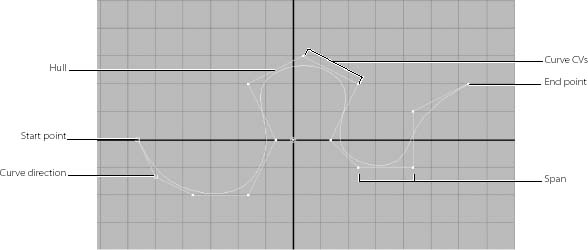
In essence, Bézier curves are created with a starting and an ending control vertex (CV) and usually two CVs in between that provide the curvature. As each CV is laid down, the curve or spline tries to go from the previous CV to the next one in the smoothest possible manner.

As shown in Figure 5.1, CVs control the curvature. The hulls connect the CVs and are useful for selecting multiple rows of CVs at a time. The starting CV appears in Maya as a closed box. The second CV, which defines the curve's direction, is an open box, so you can easily see the direction in which a curve has been created. The curve ends, of course, on the endpoint CV. The start and end CVs are the only CVs that are always actually on the curve.

Figure 5.1 A Bézier curve and its components

NURBS Modeling

NURBS surfaces are defined by curves called isoparms, which are created with CVs. The surface is created between these isoparms to form spans that follow the surface curvature defined by the isoparms, as in Figure 5.2. The more spans, the greater the detail and control over the surface—but this added detail makes greater demands on the computer, especially during rendering.

Figure 5.2 NURBS surfaces are created between isoparms. You can sculpt them by moving their CVs.

It's easier to get a smooth deformation on a NURBS surface with few CVs. Achieving the same smooth look on a polygon would take much more surface detail. As you can see in Figure 5.3, NURBS modeling yields a smoother deformation, whereas polygons can become jagged at the edges.

Figure 5.3 A NURBS cylinder (left) and a polygonal cylinder (right) bent into a C shape. The NURBS cylinder remains smooth, and the polygon cylinder shows its edges. A NURBS object retains its smoothness more easily, although it's possible to create a smooth polygon bend with increased surface faces.

If your model requires smooth curves and organic shapes, use NURBS. You can convert NURBS to polygons at any time, but converting back to NURBS can be tricky.

Try This Open a new scene (choose File New Scene). In the new scene, you'll create a few curves on the ground plane grid in the Perspective (persp) panel. Maximize the perspective view by moving your cursor to it and pressing the spacebar. Choose Create CV Curve Tool. Your cursor turns into a cross. Lay down a series of points to define a curved line on the grid. Notice how the Bézier curve is created between the points (CVs) as they're laid down.

NURBS surfaces are created by connecting (or spanning) curves. Typical NURBS modeling pipelines first involve the creation of curves that define the edges, outline, paths, and/or boundaries of surfaces.

Figure 5.4 Degrees of NURBS display smoothness.

A surface's shape is defined by its isoparms. These surface curves, or curves that reside solely on a surface, show the outline of a surface's shape much as the chicken wire in a wire mesh sculpture does. CVs on the isoparms define and govern the shape of these isoparms just as they would regular curves. Adjusting a NURBS surface involves manipulating the CVs of the object.

Levels of Detail

NURBS is a type of surface in Maya that lets you adjust its detail level at any time to become more or less defined as needed. The display detail keys (1, 2, 3) adjust the level of NURBS detail shown in the panels only.

Press 2, and you'll see the wireframe mesh get denser. Press 3, and the mesh will get even denser. You can view all NURBS objects, such as this sphere, in three levels of display. Pressing 1, 2, or 3 toggles between detail levels for any selected NURBS object, as shown in Figure 5.4.

NURBS Surfacing Techniques

The easiest way to create a NURBS surface is to create a NURBS primitive. You can sculpt the primitive surface by moving its CVs, but you can also cut it apart to create different surface swatches or patches to use as needed, which you'll see in a steam pump model for the locomotive later in this chapter. Using the surfacing tools available under the Surfaces menu set, you can detach, cut, and attach pieces into and out of a primitive to get the exact shapes you need.

You can also make surfaces in several ways without using a primitive. All these methods involve first creating or using existing NURBS curves, or curves on another surface, to define a part or parts of the surface, and then using one of the methods described in the following sections to create the surfaces.

Lofting

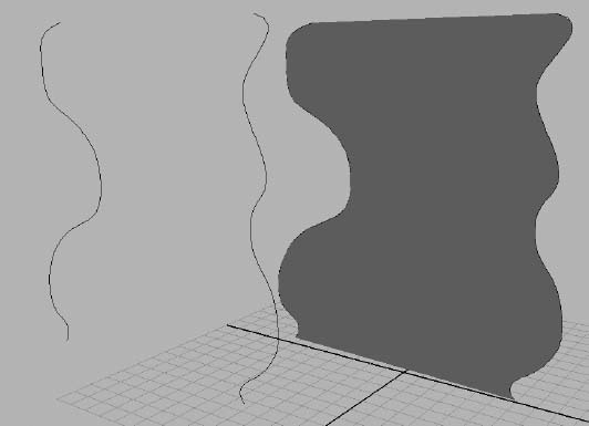
The most common surfacing method is lofting, which takes at least two curves and creates a surface span between each selected curve in the order in which they're selected. Figure 5.5 shows the result of lofting two curves together.

Figure 5.5 A simple loft created between two curves

To create a loft, follow these steps:

1. Switch to the Surfaces menu set (press F4).
2. Draw the two curves.
3. Select the curves in the order in which you want the surface to be generated.
4. Choose Surfaces Loft, or click the Loft icon in the Surfaces shelf ().

When you define more curves for the loft, Maya can create more complex shapes. The more CVs for each curve, the more isoparms you have, and the more detail in the surface. Figure 5.6 shows how four curves can be lofted together to form a more complex surface. You can use almost any number of curves for a lofted surface.

Lofting works best when curves are drawn as cross-sectional slices of the object to be modeled. Lofting is used to make a variety of surfaces, which may be as simple as tabletops or as complex as human faces.

Revolved Surface

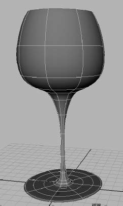
A revolved surface requires only one curve that is turned about a point in space to create a surface, like a woodworker shaping a table leg on a lathe. First you draw a profile curve to create a profile of the desired object, and then you revolve this curve (anywhere from 0 degrees to 360 degrees) around a single point in the scene to create the surface. The profile revolves around the object's pivot point, which is typically placed at the origin but can be moved (as seen in the Solar System exercise in Chapter 2, “Jumping in Headfirst, with Both Feet”), and sweeps a new surface along its way. Figure 5.7 shows the profile curve for a wine glass.

The curve is then revolved around the Y- axis a full 360 degrees to create the wine glass. Figure 5.8 is the complete revolved surface with the profile revolved around the Y-axis.

To create a revolved surface, draw and select your profile curve, and then choose Surfaces Revolve.

A revolved surface is useful for creating objects such as bottles, furniture legs, and baseball bats—anything that is symmetrical about an axis.

Figure 5.6 A loft created with four curves that are selected in order from left to right

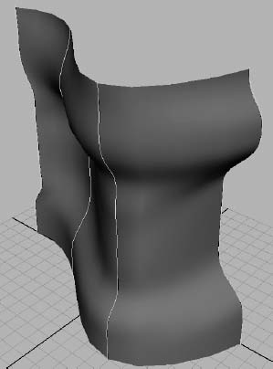
Figure 5.7 A profile curve is drawn in the outline of a wine glass in the Y-axis.

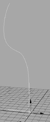
Figure 5.8 The revolved surface

Extruded Surface

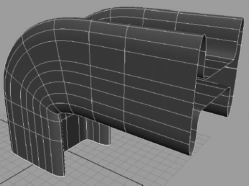
An extruded surface uses two curves: a profile curve and a path curve. The profile curve is drawn to create the profile shape of the desired surface. It's then swept from one end of the path curve to its other end, creating spans of a surface along its travel. The higher the CV count on each curve, the more detail the surface will have. An extruded surface can also take the profile curve and simply stretch it to a specified distance straight along one direction or axis, doing away with the profile curve. Figure 5.9 shows the profile and path curves, and Figure 5.10 shows the resulting surface after the profile is extruded along the path.

Figure 5.9 The profile curve is drawn in the shape of an I, and the path curve comes up and bends toward the camera.

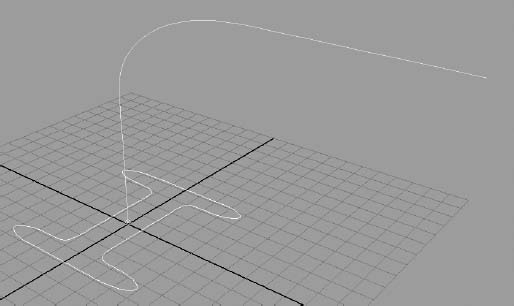
Figure 5.10 After extrusion, the surface becomes a bent I-beam.

To create an extruded surface, follow these steps:

1. Draw both curves.
2. Select the profile curve.
3. Shift+click the path curve.
4. Choose Surfaces Extrude.

An extruded surface is used to make items such as winding tunnels, coiled garden hoses, springs, and curtains.

Planar Surface

A planar surface uses one perfectly flat curve to make a two-dimensional cap in the shape of that curve. It does so by laying down a NURBS plane (a flat, square NURBS primitive) and carving out the shape of the curve like a cookie cutter. The resulting surface is a perfectly flat, cutout shape, also known as a trimmed surface because the “excess” outside the shape curve is trimmed away.

To create a planar surface, draw and select the curve and then choose Surfaces Planar.

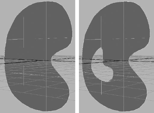
You can also use multiple curves within each other to create a planar surface with holes in it. A simple planar surface is shown on the left side of Figure 5.11. When a second curve is added inside the original curve and both are selected, the planar surface is created with a hole. On the right side is the result when the outer curve is selected first and then the inner curve is selected before Surfaces Planar is chosen.

Figure 5.11 A planar surface based on a single curve (left). A planar surface based on a curve within a curve to create the cutout (right).

A planar surface is great for flat lettering, for pieces of a marionette doll or paper cutout, or for capping the ends of a hollow extrusion. Planar surfaces are best left as flat pieces, however, because deforming them may not give the best results. In addition, it's sometimes best to create the planar surface as a polygon. You'll see how to convert surfaces to polygons later in this chapter. The following quick exercise will give you an idea of what to look out for when creating polygons from surfacing techniques:

1. In the Surfaces menu set, select Create NURBS Primitives Circle twice to create two circles.
2. Scale the second circle to about three times its original size, as shown in Figure 5.12.
3. Select the larger circle first, then the smaller circle, and finally select Surfaces Planar . In the option box, check Polygons for Output Geometry, Quads for Type, and General for Tessellation Method, as shown in Figure 5.13.
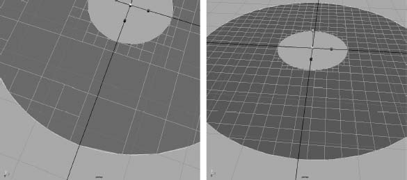
4. Depending on how you create the geometry as polygons, you'll get different results—particularly around curves. Because Maya has to figure out where to put more faces to create a smoother outline, you have to set the Number U and Number V settings to best fit the curves of your resulting surface. At the current settings, your planar surface looks as shown in Figure 5.14. Notice the small gaps between the original outer NURBS circle and the surface outline.
5. Increase the Number U and Number V values, and you'll get tighter results at curves, although you'll have more faces on your model.

Figure 5.12 Scale the circle up.

Figure 5.13 Choose these options.

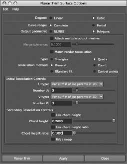
Figure 5.14 Notice the gaps between the outer NURBS circle and the outline.

Keep this exercise in mind as you continue modeling. Whenever you need to create polygons from NURBS surfaces—which should be quite often for some people—try the different creation methods for the best output. No one way works best all the time.

Figure 5.15 A curve before and after it's beveled. The beveled surface has been given a planar cap.

Beveled Surface

The Bevel Surface function takes an open or a closed curve and extrudes its outline to create a side surface. It creates a bevel on one or both corners of the resulting surface to create an edge that can be made smooth or sharp (see Figure 5.15). The many options in the Bevel tool allow you to control the size of the bevel and depth of extrusion, giving you great flexibility. When a bevel is created, you can easily cap the bevel with planar surfaces.

To create a bevel, draw and select your curve, and then choose Surfaces Bevel.

Maya also offers a Bevel Plus surface, which has more creation options for advanced bevels. A beveled surface is great for creating 3D lettering, for creating items such as bottle caps or buttons, and for rounding out an object's edges.

Boundary Surface

A boundary surface is so named because it's created within the boundaries of three or four surrounding curves. For example, two vertical curves are drawn opposite each other to define the two side edges of the surface. Two horizontal curves are then drawn to define the upper and lower edges. These curves can have depth to them; they need not be flat for the boundary surface to work, unlike a planar surface. Although you can select the curves in any order, it's best to select them in opposing pairs. In Figure 5.16, four curves are created and arranged to form the edges of a surface to be created. First, select the vertical pair of curves, because they're opposing pairs; then, select the second two horizontal curves before choosing Surfaces Boundary.

A boundary surface is useful for creating shapes such as car hoods, fenders, and other formed panels.

Figure 5.16 Four curves arranged to create the edges for a surface (left). The resulting boundary surface formed from the four curves (right).

Combining Techniques

You can use certain surfacing techniques in combination to create intricate models. For example, whenever a curve is required for a surface, you can use an isoparm instead to create a surface between two existing surfaces.

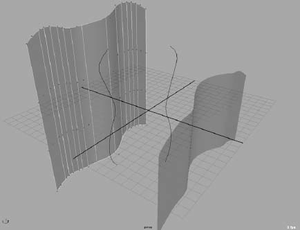
Try This Take a couple of lofted surfaces, and connect them with a third surface. Figure 5.17 shows two surfaces with two intermediate curves between them. (Notice that the view panel's option Shading X-ray is turned on so you can see through the shaded surfaces.) You'll select an isoparm from the first surface (on the left) and then the curve on the left, the curve on the right, and finally an isoparm on the second surface:

1. Either create two lofted surfaces and curves as shown in Figure 5.13, or load the Chap_5_Lofting_Exercise_1.ma file from the Lofting_Exercise project on the book's companion web page, www.sybex.com/go/intromaya2012.

   Figure 5.17 Two lofted surfaces with two curves in between

   

2. To select the first isoparm, press F8 for Component Selection mode, and click the Lines Selection Filter button () in the Status line to allow you to select isoparms. You can also right-click the surface and choose Isoparm from the marking menu to enter Component Selection mode for isoparms.
3. Select an isoparm close to the left edge. Press F8 to return to Object Selection mode (or right-click the first curve and choose Object Mode from the marking menu), Shift+click the first curve, and then Shift+click the second curve. Press F8 again or use the marking menu again for Component Selection mode, and Shift+click an isoparm toward the left edge on the second surface, as in Figure 5.18.

   Figure 5.18 Selecting the isoparm

   

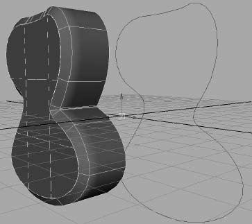
4. Choose Surfaces Loft to create the intermediate surface between the existing lofts. Figure 5.19 shows how the new surface snakes from the first loft to the second loft by way of the two curves.

Figure 5.19 The spanning loft between the existing surfaces snakes from the first isoparm to the curves to the second isoparm.

Surface History

In Chapter 3, “The Maya 2012 Interface,” you learned that clicking the History icon () toggles History on and off. History has to do with how objects react to change. Leaving History on when creating primitives, as you did in Chapter 2, allows you to access an object's original parameters.

Leaving History on when creating NURBS surfaces allows the surface to update when any of its creation pieces change. For example, the loft you just created will update whenever the two original surfaces or curves you used to create the loft move or change shape. If you were to move the original loft on the left and rotate it back a bit, the new loft would adjust to keep its one side attached to the same isoparm. If one or more of the input curves were to change, the loft would bend to fit.

By lofting using isoparms and with History toggled on, you can keep the new surface permanently attached to the original loft, no matter how the isoparms move, as in Figure 5.20. This technique works with all surface techniques, not just with lofting, as long as History is turned on. History is useful for making adjustments and fine-tuning a surface, and it can be handy in animation if several surfaces need to deform but stay attached.

Figure 5.20 History updates the newly created loft to keep it attached to the isoparms and curves used to create it, even when they've been moved or altered.

Why wouldn't you want History turned on for everything? After a long day of modeling, having History on for every single object can slow down your scene file, adding unnecessary bloat to your workflow. But it isn't typically a problem on most surface types unless the scene is huge, so you should leave it on while you're still modeling.

If you no longer want a surface or an object to retain its History, you can selectively delete it from the surface. Select the surface, and choose Edit Delete By Type History. You can also rid the entire scene of History by choosing Edit Delete All By Type History. Just don't get them mixed up!

Using NURBS Surfacing to Create Polygons

You can create swatches of polygon surfaces by using NURBS surfacing tools, as you saw during the exercise on creating a planar surface.

To create a polygonal surface with any of the surfacing techniques in this chapter, open the option box for that particular NURBS tool. For example, create two simple curves. With both curves selected, choose Surfaces Loft . In the options for Output Geometry, click the Polygons button to display the options for creating the polygon surface and its detail level.

History for the surface will adjust the new polygonal surface. The detail of the surface will try to adjust as changes to the input curves are made. If you anticipate significant changes to the input curves, make sure you create the poly surface with a high poly count to accommodate major changes. This is probably the best way to create a single poly surface, especially if you prefer a NURBS workflow.

Try This Draw two CV curves as you did at the beginning of this chapter, both with the same number of CVs. Open the Loft option box, and click the Polygons option for the Output Geometry.

The creation options that appear at the bottom of the window affect the tessellation of the resulting surface; that is, you use them to specify the level of detail and the number of faces with which the surface is created. Generally speaking, the more faces there are, the more detail you'll need. (That doesn't mean a detailed surface can't be efficient, with areas of high tessellation placed only where needed.)

The default Tessellation Method, Standard Fit, uses the fewest faces to create the surface without compromising overall integrity. The sliders adjust the resulting number of faces in order to fit the finer curvature of the input curves.

The lower the Fractional Tolerance, the smoother the surface and the greater the number of faces you need.

The Chord Height Ratio determines the amount of curve in a particular region and calculates how many more faces to use to give an adequate representation of that curved area with polygons. This option is best used with surfaces that have multiple or very intense curves.

It isn't uncommon to create a surface, undo it, change the slider settings, re-create it, and repeat, to get just the right tessellation. That's why you should click the Apply button, which keeps the window open, rather than the Loft button, which closes the window after applying the settings.

The General Tessellation Method creates a specific number of lines, evenly dividing the horizontal (U) and vertical (V) into rows of polygon faces.

The Control Points method tessellates the surface according to the number of points on the input curves. As the number of CVs and spans on the curves increases, so does the number of divisions of polygons.

The Count method simply relies on how many faces you tell it to make—the higher the count, the higher the tessellation on the surface. Experiment with the options to get the best poly surface results.

Converting a NURBS Model to Polygons

Some people prefer to model on NURBS curves and either create poly surfaces or convert to polygons after the entire model is done with NURBS surfaces. Ultimately, you'll find your own workflow preference, but it helps greatly if you're comfortable using all surfacing methods. Most modelers choose one way or another but are familiar with both methodologies. In the following section, you'll convert a NURBS model to polygons.

Try This Convert a NURBS modeled axe into a poly model like one that might be needed in a game.

Open axe_model_v1.mb in the Scenes folder of the Axe project from the companion web page. The toughest part of this simple process is getting the poly model to follow all the curves in the axe with fidelity, so you'll have to convert parts of the axe differently. Follow these steps:

1. Grab the handle, and choose Modify Convert NURBS to Polygons . Use the default presets. If need be, reestablish your settings by choosing Edit Reset Settings; the handle converts well to polygons. Click Apply, and a poly version of the axe handle appears on top of the NURBS version. Move it eight units to the right to get it out of the way. You'll move the other parts 8 units as well to assemble the poly axe properly.
2. Select the back part of the axe head. All those surfaces are grouped together to make selection easy. The default settings will work for this part as well, so click Apply and move the resulting model eight units to the left.
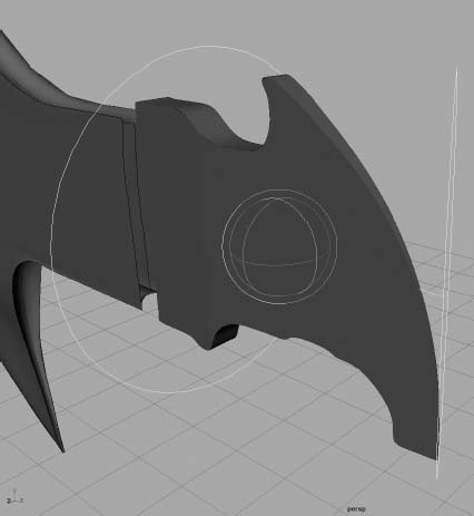
3. The front of the axe head holds a lot of different arcs, so you'll have to create it with finer controls. Change Fractional Tolerance from 0.01 to 0.0005. This yields more polygons but finer curved surfaces. Figure 5.21 shows the result.

Figure 5.21 A faithful high-poly conversion (on the right) of a NURBS axe (on the left)

If you were following this process for a conventional game engine, you'd normally be restricted to a low number of polygons, and your axe design would be different to better handle a low poly count.

Editing NURBS Surfaces

As you've experienced, Maya provides numerous NURBS tools that you'll find useful when editing your surfaces. In addition to tools for moving CVs, some important functions and tools allow you to add realism to your model. This section gives you a quick overview of these tools—some you've already used, and others you'll need to try out for yourself.

The following functions are all accessed through the Edit NURBS menu. Open and tear off the Edit NURBS menu so it remains open as you follow along.

Project Curve on Surface

The ability to project a curve onto a surface allows you to cut holes in the surface using the Trim tool (choose Edit NURBS Trim Tool). It also lets you create, using History, another surface that is attached, following the outline of your projected curve, as you saw in the section “Combining Techniques” earlier in this chapter.

Similar to drawing a curve on a surface, projected curves project an existing curve onto the selected surface. That curve on the surface is now useful for patch modeling as well as tracing animation paths for objects to follow along a surface. For example, you can project a curve around a hilly landscape surface and assign a car to animate (drive) along that projected curve. The car will stick to the surface of the road with ease.

To use Project Curve On Surface, select the surface and the curve to project, and then choose Edit NURBS Project Curve On Surface.

Trim and Untrim Surfaces

Trimming a surface (choose Edit NURBS Trim Tool) creates holes in the surface using curves that are either drawn or projected onto the surface.

If you have a surface that has already been trimmed, and it's too late to reverse the function with Undo, you can use Untrim Surfaces to remove either the last trim performed or all the surface trims. Choose Edit NURBS Untrim Surfaces.

Attach Surfaces

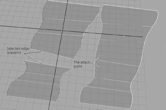
Attach Surfaces does exactly that—it attaches two contiguous NURBS surfaces along two selected isoparms. Select an isoparm on the edge of the first surface, Shift+click an edge isoparm on a second surface, and choose Edit NURBS Attach Surfaces to create a new surface from the two. As shown in Figure 5.22, the attach point is along the selected isoparms.

Figure 5.22 Attach Surfaces connects surfaces along their selected isoparms.

Detach Surfaces

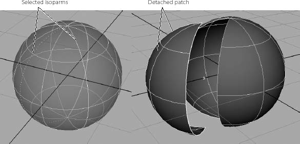
Detach Surfaces is a highly useful tool for generating specific areas of a NURBS surface, or patches. Select an isoparm to define the line of detachment, and choose Edit NURBS Detach Surfaces. The surface is cut along that isoparm to create two distinct surfaces (see Figure 5.23). You'll see plenty of Detach and Attach tools later in this chapter.

Figure 5.23 Detach Surfaces cuts a surface at the selected isoparms to create a new surface.

Insert Isoparms

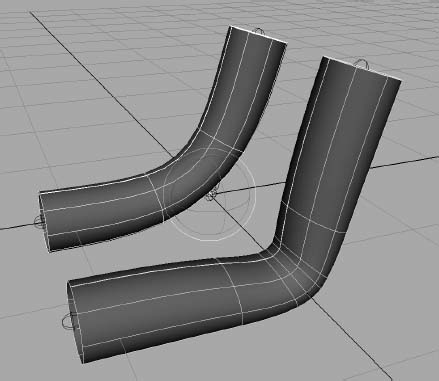
Adding extra surface definition by adding spans is a matter of selecting an isoparm and choosing Edit NURBS Insert Isoparms. This creates an isoparm and redefines the surface to add more spans to allow for smoother deformations—for example, adding an isoparm or two to the elbow joint of a model to make the arm bend with a cleaner crease (see Figure 5.24). You can either create a new isoparm between two existing ones or add isoparms to your own defined area.

Figure 5.24 Inserting isoparms for a smoother deformation

Patch Modeling: A Locomotive Detail

With NURBS modeling, you frequently need to attach surfaces so that a model doesn't split at the seams. This process of aligning and attaching NURBS patches is called stitching, and this kind of modeling is called patch modeling.

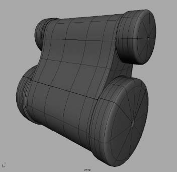
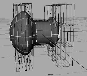
Figure 5.25 The finished pump elements for the previous chapter's locomotive model are created in NURBS patches.

We're jumping back in time to create a pump for the polygonal locomotive you made in Chapter 4, “Beginning Polygonal Modeling.” You will use patches that you'll stitch together. This exercise gives you an idea of how patches work to pull together an organic shape using NURBS shapes. To show you what you're seeking to build, the finished model is shown in Figure 5.25.

Keep in mind that patch modeling is a fairly involved process. If you don't feel comfortable with modeling quite yet, skip this exercise and move on to the next section in this chapter, “Using Artisan to Sculpt NURBS.” You can always return to this section to bone up on your patch modeling later.

Starting the NURBS Pump

First, create a new project called Locomotive, or copy the Locomotive project from the companion web page to your hard drive and set it as your current project.

To start creating the locomotive pump, follow these steps:

1. Create a NURBS cylinder with no caps by choosing Create NURBS Primitives Cylinder . Under Caps in the option box, select None to create an open-ended cylinder. Set Axis to Z to create the cylinder on its side, and then click Create.
2. Size the cylinder down to 0.72 in X and Y and to 0.9 in Z.
3. Reset the cylinder so that its attributes are set back to normal. With the cylinder selected, choose Modify Freeze Transformations . In the option box, choose Edit Reset Settings to set to reestablish the defaults, and then click Freeze Transform. The cylinder, resized and after the application of Freeze Transformations, is shown in Figure 5.26.
4. You'll create slightly larger end pieces for the cylinder. Duplicate the cylinder once, move the copy, and scale it as shown in Figure 5.27. Repeat to create the other end piece. The end pieces are roughly 1.075 in Scale X and Y and 0.18 in Scale Z and are moved slightly past the ends of the cylinder, leaving a slight gap as shown. You should freeze transforms on the ends to reset their scale and positions back to the default.
5. Create a second copy of this assembly that is smaller in radius but is the same length (see Figure 5.28). Duplicate the three cylinders, and change their respective scales to 0.55 in X and Y but leave Scale Z set to 1. Remember, you froze their transforms, so their starting scales should have been at 1. Position the three cylinders as shown in Figure 5.28, slightly to the side and above the original larger cylinders. Freeze their transforms.

   Figure 5.26 The first NURBS cylinder, after Freeze Transformations

   

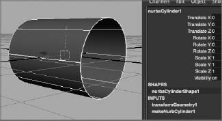
   Figure 5.27 Create the end pieces.

   

6. Cut a couple of holes in the main cylinders. Cut at the top two isoparms on the sides of the larger cylinder first, as shown in Figure 5.29. To select the first isoparm, right-click the cylinder, choose Isoparm from the marking menu, and click the isoparm to select it. Next, Shift+click the isoparm on the other side so that both are selected.
7. In the Surfaces menu set, choose Edit NURBS Detach Surfaces. The surface between the isoparms you just selected is now its own surface and can be deleted. This gives your first cut, as shown in Figure 5.30.
8. Use the same procedure to cut the smaller cylinder, but at the sides so you can remove the bottom half. Select the isoparms on the sides of the smaller cylinder, and detach the surface by choosing Edit NURBS Detach Surfaces again. Delete the bottom surface. Now your model should look like Figure 5.31.

Figure 5.28 Create a smaller copy of the first cylinders, and place them higher for the top of the steam pump assembly.

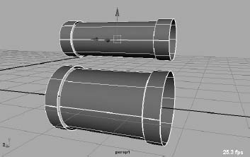
Figure 5.29 Select these isoparms to cut the top of the cylinder.

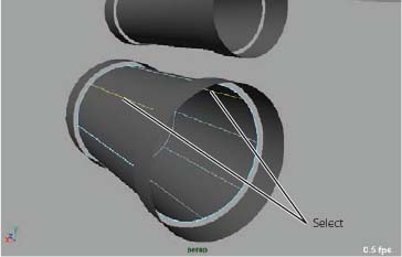
Figure 5.30 Cutting the cylinder's top

Figure 5.31 The cut cylinders

Adding End Caps

At this point, you'll cap the ends of the cylinders to close them off. You can continue with your own file or load the file NURBS_pump_v01.mb from the Locomotive project from the companion web page and check your work so far. The trick will be to add four isoparms using the Insert Isoparms function you read about earlier in this chapter to create the caps.

To cap the ends, follow these steps:

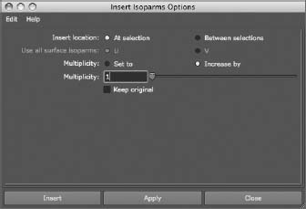
1. Select the end cylinder, right-click the geometry, and select Isoparm from the marking menu. Select four isoparms (make sure you hold down Shift while selecting the isoparms so as not to deselect them), as shown in Figure 5.32, and choose Edit NURBS Insert Isoparms .

   Make sure your settings match those in Figure 5.33. This inserts four isoparms into the end cylinder that you can use to close the end to make the cap.

   Figure 5.32 Select these four isoparms.

   

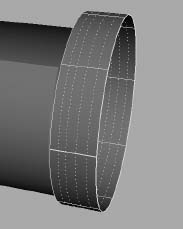
   Figure 5.33 The default Insert Isoparms settings

   

2. Select the end CVs to scale them down to close the cap. The easiest way to do this is to select the hull that controls all the edge CVs. Right-click the end cylinder and select Hull. Select the very outermost hull, and scale it down as shown in Figure 5.34. Doing so closes the end cap. Don't worry about leaving a small hole in the cap; you'll complete this pump when you finish the locomotive model.
3. Repeat the previous procedures to close off the other three end cylinders to create caps for both ends of both objects, as shown in Figure 5.35.

   Figure 5.34 Scale down the outermost hull.

   

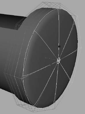
   Figure 5.35 End caps for the pump pieces

   

4. Connect and patch the end caps to their cylinders. To do this, you need to line up a few new isoparms on the cylinders so you can stitch everything together properly. Using the previous workflow, add new isoparms to the bottom cylinder, as shown in Figure 5.36. (You may have to hide the end caps to create the isoparms on the cylinder. Select the end caps and use Display Hide Hide Selection. After you create the isoparms, select Display Show All.)

   Figure 5.36 Add isoparms as shown here.

   

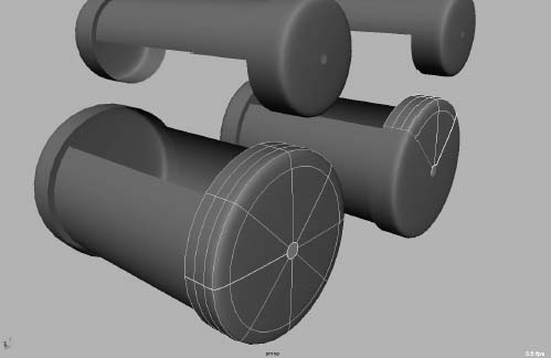
5. You need to prep the end cap to connect to the cylinder, by cutting a pie piece out of the cap, to line it up with the cut cylinder. On the end cap, select two isoparms to form a V that lines up with the cut edges of the main cylinder, as shown in Figure 5.37. Then, choose Edit NURBS Detach Surfaces. Doing so cuts the V section out of the end cap. This aligns the end cap and the cylinder geometry at the edges so you can create a smooth connection between them in the next few steps.

   Figure 5.37 Select two isoparms and detach the surfaces.

   

   You can load the file NURBS_pump_v02.mb from the Locomotive project to compare your work with it. Or, if you skipped the previous steps, you can proceed from here to attach the end cap.

6. You need to pull the end of the cylinder to line it up with the edge of the end cap. Select the end four vertical hulls, as shown in Figure 5.38, and move them so that the edges of the cylinder and end cap align. Repeat this to line up the other end of the cylinder with the other cap.
7. Create the pieces to connect the caps to the cylinder using lofts. Right-click the cylinder, and choose Isoparm from the marking menu. Select the edge isoparm on the cylinder. Right-click the end cap, and choose Isoparm from the marking menu. Shift+click the edge isoparm of the end cap, as shown in Figure 5.39. Choose Surfaces Loft . Make sure you're using the default settings for the loft: in the option box, choose Edit Reset Settings.
8. The previous step creates a surface to bridge the cylinder and the end cap. You'll notice that it's rather jagged—almost a diamond shape as opposed to a smooth ring. With the loft selected, press 3 on the keyboard to see it with a smooth display in the panel. Figure 5.40 shows the loft.

Figure 5.38 Select the four end hulls and move them to line up.

Figure 5.39 Shift+click the edge isoparm.

Figure 5.40 Lofting the end cap to the cylinder

Stitching and Tangency

Smooth seams are essential to organic modeling. The trick in creating a good patch model is to make sure all the patches line up; this is called tangency. In animation and texture setup, it's important that tangency be correct; otherwise, you may notice tearing at seams during deformations or texture maps that don't line up quite right. It can be a tedious process, but here is a taste of it. To continue with the patch model of the locomotive pump, follow these steps:

1. Create a smooth piece that connects the cylinder and the end caps using the lofts created in steps 7 and 8 in the previous section and shown in Figure 5.40. Select the cylinder and the connector loft, as shown in Figure 5.41, and attach them by choosing Edit NURBS Attach Surfaces . Make sure the tool is set to the default (choose Edit Reset Settings). Turn off Keep Originals and click Attach. This blends the two surfaces into one, creates a smooth transition between them, and deletes the original surfaces.
2. Here's the funny part: You need to disconnect the surfaces. Select the isoparm at the location where the patches originally met, and choose Edit NURBS Detach Surfaces. Again, make sure the tool is reset to the default so as not to keep the original patches. This gives you tangency across the two patches as well as a smooth transition in the model.
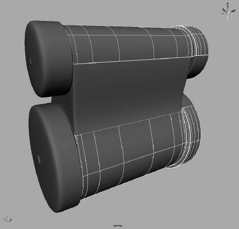
3. Repeat steps 1 and 2 for the other end of the cylinder and its end cap and also for the upper cylinder and its two end caps. You should now have end caps with smooth attachments to the cylinders, as shown in Figure 5.42.

   Figure 5.41 Attach the patches.

   

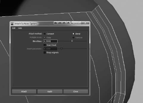
   Figure 5.42 The end caps attach to the cylinders—smooth as low-cholesterol butter!

   

4. Connecting the upper and lower cylinders is next. Select the edge isoparms of both cylinders, and choose Surfaces Loft . Set the Section Spans to 2 in the option box and click Apply. Repeat to create a loft on the back side of the cylinders as well. Figure 5.43 shows the resulting surfaces.

   Figure 5.43 Lofting the two cylinders together

   

5. Individually select the middle hulls of both of the lofts, and move them back to create a bit of curvature to the surfaces, as shown in Figure 5.44. Remember, you can select hulls by right-clicking the surface and using the marking menu.

   Figure 5.44 Move back the middle and lowermiddle hulls.

   

6. Select the edge isoparms of the lofts you just created, and loft between them with two spans. Make sure you reset the loft settings by choosing Edit Reset Settings in the option box, and then set Section Spans to 2 spans before you create the loft. Repeat for the other side. Figure 5.45 shows the closed ends.

   Figure 5.45 Closing the sides

   

7. Go into CV mode, and move the CVs to line up the edges of the newly formed closed ends with the bottom and top cylinders. Repeat for the other side, as shown in Figure 5.46.

   Figure 5.46 In CV mode, line up the ends and cylinders.

   

8. As you did in steps 1 and 2, attach and then detach the loft you just edited with CVs (we'll call it the side panel) and the front panel, as shown in Figure 5.47, to set up a smooth transition and a tangency. Repeat for the back panel and the other end of the cylinders to make the other side panel.
9. Shift your attention to one of the end caps on the lower cylinder. In step 5 in the previous section, and as shown in Figure 5.37, you detached a pizza-slice shape out of the end caps. Select the detached slice, and insert two isoparms between the existing ones. Your model should resemble the one in Figure 5.48 with the added isoparms. This is set up for another attachment in a moment. Repeat for the other end cap on the lower cylinder.

   

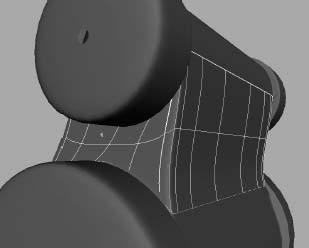
   Figure 5.47 Create a smooth transition between the surfaces.

   

   Figure 5.48 Insert isoparms into the end cap slice.

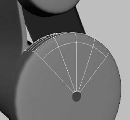
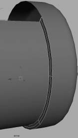
10. Select isoparms on the edges of the end cap and the side panel, and loft between them with two spans. Repeat for the other side. Doing so plugs the hole between the end cap and the side panels. You can, if you like, run another attach and detach to smooth out the groove between the end caps and the side panels. Figure 5.49 shows the end result of the groove.
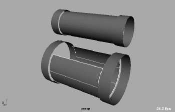
11. You're getting kicked out into the cold now to run the same set of procedures on the upper cylinder and its end caps. These should be simpler, because there are fewer sections to deal with. Go ahead and finish the model from here to form the connections shown in Figure 5.50 and to form the final model shown in Figure 5.51.

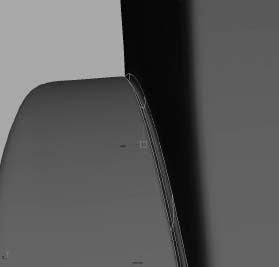
Figure 5.49 The groove connecting the end cap with the side panel

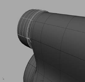
Figure 5.50 Finishing the top part of the NURBS pump

There is quite a bit of lofting, attaching, and detaching between surface patches in patch modeling. The key to becoming good at it is to be able to line up isoparms easily and cleverly and to be able to attach them again smoothly; it takes a lot of practice to get used to this technique. You'll make a lot of mistakes along the way, but that is how you'll learn the most! It's easy to see how this kind of modeling is useful for making organic shapes such as faces.

Figure 5.51 The finished pump

Using Artisan to Sculpt NURBS

Imagine that you can create a NURBS surface and sculpt it using your cursor the way hands are used on wet clay to mold the surface. You can do just that with a Maya module called Artisan—and without the mess!

Try This Artisan is basically a 3D painting system that allows you to paint directly onto a surface. By painting on the surface with the Sculpt Geometry tool, you move the CV points in and out, effectively molding the surface.

1. In Shaded mode (press 5), maximize the Perspective window (press the spacebar) for a nice big view. Create a NURBS sphere, and open the Attribute Editor. In the sphere's creation node (makeNurbsSphere1), set Sections to 24 and Spans to 12. The greater the surface definition, the more detailed the sculpting.
2. Select the sphere, and choose Edit NURBS Sculpt Geometry Tool . Clicking the option box opens the tool settings. You'll need those almost every time you paint with Artisan to change brush sizes and so forth.

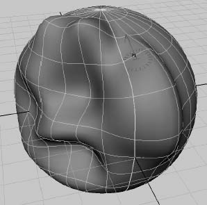
   Your cursor changes to the Artisan brush, as shown in Figure 5.52. The red circle around the brush cursor and the lettering displays the type of brush you're currently using. When the red lines point outside the circle and the lettering reads Ps, you're using the push brush that pushes in the surface as you paint it. The black arrow pointing toward the sphere's center is a measurement of the Max Displacement slider in the tool settings. This sets how far each stroke pushes in the surface. The lower the number, the less the brush affects the surface.

3. Click and drag the cursor across the surface of the sphere to get a feel for how the surface deforms under your tool. Use the Max Displacement slider to control the force of the brush, and use Radius (U) and Radius (L) to set the size of the brush.
4. Switch your brush type to pull. Your cursor changes to read Pl, and the red lines appear on the inside of the circle (see Figure 5.53). You can then pull out the surface.

   Figure 5.52 The Sculpt Geometry tool lets you mold your surface by painting on it. Here the brush is set to push in the surface of the sphere as you paint.

   

   The Opacity slider also controls the force of the brush, but it's subtler than Max Displacement to give you greater control. Because this is after all a 3D painting tool, Opacity controls how much value you paint onto the surface. The value in this case isn't a color but how far the surface is deformed. You'll see how Artisan comes into play in other aspects of Maya later in the book.

5. Smooth blends the pushed-in and pulled-out areas of the surface to yield a smoother result. Erase simply erases the deformations on the surface, setting it back to the way it was before.

Figure 5.53 With a pull brush, your cursor changes to read Pl.

If you plan to sculpt a more detailed surface, be sure to create the surface with plenty of surface spans and sections. If you only want to paint a specific area of a NURBS surface, choose Edit NURBS Insert Isoparms to add extra detail to that area before you begin painting, although you can add isoparms after you paint. When you begin to sculpt this way, going back into the surface's creation node to increase its sections and spans will ruin your results.

Modeling with Simple Deformers

In many ways, deformers are the Swiss Army knives of Maya animation, except you can't open a bottle with them. Deformers are handy for creating and editing modeled shapes in Maya. These tools allow you to change the shape of an object easily. Rather than using CVs or vertices to distort or bend an object manually, you can use a deformer to affect the entire object. Popular deformers, such as Bend and Flare, can be powerful tools for adjusting your models quickly and evenly, as you're about to see.

Nonlinear deformers, such as Bend and Flare, create simple shape adjustments for the attached geometry, such as bending the object. You can also use deformers in animation to create effects or deformations in your objects. We'll explore this later in the book.

Modeling Using the Bend Deformer

Let's apply a deformer. In a new Maya scene, you'll create a polygonal cylinder and bend it to get a quick idea of how deformers work. Follow these steps:

1. Choose Create Polygon Primitives, and turn on Interactive Creation. Then, choose Create Polygon Primitives Cylinder. Click and drag to create the base. Make it a few units in diameter; the exact sizing isn't important here. Click and drag to make the height of the cylinder 7 or 8 units, as shown in Figure 5.54. Make sure your create options are set to the defaults so that they're consistent with these directions.

   To make sure the settings are at their defaults, open the command's option box and click the Reset Settings button.

2. Let's jump right in and create the Bend deformer. With the cylinder selected, switch to the Animation menu set by pressing F2 and choosing Create Deformers Nonlinear Bend. Your cylinder turns magenta, and a thin line appears at the center of the cylinder, running lengthwise. Figure 5.55 shows the deformer and its Channel Box attributes. Depending on your settings, your deformer may be created in a different axis than the one pictured. You can reset the deformer's options as needed. Click bend1 in the Channel Box to expand the deformer's attributes shown in the figure.

   

   Figure 5.54 Create a cylinder to bend.

   

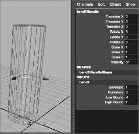
   Figure 5.55 Creating the Bend deformer

   

   Figure 5.56 Notice the problem with this cylinder?

3. Click Curvature, and enter a value of 1. Notice that the cylinder takes on an odd shape, as shown in Figure 5.56. The Bend deformer itself is bending nicely, but the geometry isn't. As a matter of fact, the geometry is now offset from its original location. It's offset because there aren't enough divisions in the geometry to allow for a smooth bend.
4. Select the cylinder, and click polyCylinder1 in the Channel Box to expand the shape node's attributes. Enter a value of 12 for the Subdivisions Height attribute (see Figure 5.57), and your cylinder will bend with the deformer properly, as shown in Figure 5.58.

   

   Figure 5.57 Increase Subdivisions Height to 12.

5. Try adjusting the Bend deformer's Low and High Bound attributes. This allows you to bend one part of the cylinder without affecting the other. Figure 5.59 shows the cylinder with the Bend deformer's High Bound set to 0.25 instead of 1. This causes the top half of the cylinder to bend only one quarter of the way up and continue straight from there.

Experiment with moving the Bend deformer, and see how doing so affects the geometry of the cylinder. The deformer's position plays an important role in how it shapes an object's geometry.

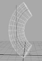
Figure 5.58 The cylinder bends properly now that it has the right number of divisions.

Figure 5.59 Using the High Bound to change the effect of the Bend deformer

Adjusting an Existing Axe Model

In this exercise, you'll take an existing NURBS model of an axe and fine-tune the back end of the axe head. In the existing model, the back end of the axe head is blunt, as you can see in Figure 5.60. You'll need to sharpen the blunt end with a nonlinear deformer. Open the AxeHead_v01.ma file in the Scenes folder of the Axe project from the companion web page, and follow these steps:

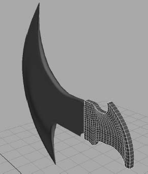
Figure 5.60 The axe head is blunt.

1. Select the top group of the axe head's back end. To do so, open the Outliner, and select axeHead_Back (see Figure 5.61).
2. Press F2 to switch to the Animation menu set.
3. Create a Flare deformer by choosing Create Deformers Nonlinear Flare. The Flare deformer appears as a cylindrical object (see Figure 5.62).
4. Rotate the deformer 90 degrees in the Z-axis, as shown in Figure 5.63.
5. Open the Attribute Editor (Ctrl+A), click the flare1 tab to access the Flare controls, and enter the following values:

Attribute	Value
Start Flare Z	0.020
High Bound	0.50

These values taper in the end of that part of the axe head, as shown in Figure 5.64. This is a much easier way of sharpening the blunt end than adjusting the individual CVs of the NURBS surfaces.

Deformers use History to distort the geometry to which they're attached. You can animate any of the attributes that control the deformer shapes, but in this case you're using the deformer as a means to adjust a model. When you get the desired shape, as shown in Figure 5.65, you can discard the deformer. However, simply selecting and deleting the deformer will reset the geometry to its original blunt shape. You need to pick the axeHead_Back geometry group (not the deformer) and delete its History by choosing Edit Delete By Type History.

Figure 5.61 Select the back of the axe head.

Figure 5.62 The Flare deformer appears as a cylinder.

Figure 5.63 Rotate the deformer 90 degrees in the Z-axis.

Figure 5.64 Sharpen the axe's back edge.

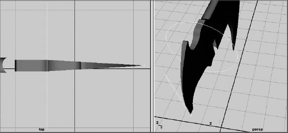
Figure 5.65 Another view of the back of the axe head with the Flare deformer

The Lattice Deformer

A simple deformer, such as a Bend or Flare, will get you only so far; when a model requires more intricate editing with a deformer, you'll need to use a lattice.

A lattice is a scaffold that fits around your geometry. The lattice object controls the shape of the geometry. When a lattice point is moved, the lattice smoothly deforms the underlying geometry. The more lattice points, the greater control you have. The more divisions the geometry has, the more smoothly the geometry will deform.

Lattices are especially useful when you need to edit a relatively complex poly mesh or NURBS surface that is too dense to edit efficiently directly with CVs or vertices. With a lattice, you don't have to move the individual surface points.

Lattices can work on any surface type, and a single lattice can affect multiple surfaces simultaneously. You can also move an object through a lattice (or vice versa) to animate a deformation effect, such as a golf ball sliding through a garden hose.

Creating an Alien Hand

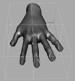
Make sure you're in the Animation menu set. To adjust an existing model or surface, select the model(s) or applicable groups to deform, and choose Create Deformers Lattice. Figure 5.66 shows a polygonal hand model with a default lattice applied. The top node of the hand has been selected and the lattice applied.

Figure 5.66 A lattice is applied to the polygonal hand model.

To experience how this works, you'll remodel the poly hand using a few different lattices. Your objective is to create an alien hand by thinning and elongating the hand and each of the fingers—we all know aliens have long gawky fingers. Because it would take a lot of time and effort to achieve this by moving the vertices of the poly mesh, using lattices here is ideal.

To elongate and thin the entire hand, load the scene file detailed_poly_hand.ma from the Poly_Hand project from the companion web page, and follow these steps:

1. Select the top node of the hand (poly_hand) in the Outliner, and choose Create Deformers Lattice. Doing so creates a default lattice that affects the entire hand, fingernails and all, as shown in Figure 5.66. Although you can change the lattice settings in the option box upon creation, you'll edit the lattice after it's applied to the hand.
2. The lattice is selected after it's created. Open the Attribute Editor, and click the ffd1LatticeShape tab. The three attributes of interest here are S Divisions, T Divisions, and U Divisions. These sliders control how many divisions the lattice uses to deform its geometry. Set S Divisions to 3, T Divisions to 2, and U Divisions to 3 for the result shown in Figure 5.67.

   Figure 5.67 Changing the number of divisions in the lattice

   

   A 3 × 2 × 3 lattice refers to the number of division lines in the lattice as opposed to the number of sections; otherwise, this would be a 2 × 1 × 2 lattice!

3. With the lattice selected, press F8 to switch to Component mode and display the lattice's points. These points act just like the vertices on a polygonal shape. You'll use them to change the overall shape of the hand without moving the vertices of the hand. Select the vertices on the thumb side of the hand, and move them to squeeze in that half of the hand. Notice how only that zone of the model is affected by that part of the lattice.

   Figure 5.68 Lengthen the hand using the deformer.

   

4. Toggle back to Object mode (press F8 again), and scale the entire lattice to be thinner in the Z-axis and longer in the X-axis. The entire hand is deformed in accordance with how the lattice is scaled (see Figure 5.68).
5. Now that you've altered the hand, you have no need for this lattice. If you delete the lattice, the hand will snap back to its original shape. You don't want this to happen. Instead, you need to delete the construction history on the hand to get rid of the lattice, as you did with the axe head exercise earlier in this chapter.

   Select the top node of the hand, and choose Edit Delete By Type History.

Creating Alien Fingers

The next step is to elongate the individual fingers and widen the knuckles. Let's begin with the index finger. Follow these steps:

1. Select the top node of the hand, and create a new lattice as before. It forms around the entire hand.

   Although you can divide the lattice so that its divisions line up with the fingers, it's much easier and more interactive to scale and position the entire lattice so it fits around the index finger only.

   Figure 5.69 Select the lattice and base nodes.

   

2. Simply moving and scaling the selected lattice will deform the hand geometry. You don't want to do this. Instead, you need to select the lattice and its base node. This lets you change the lattice without affecting the hand. In the Outliner, select both the ffd1Lattice and ffd1Base nodes (see Figure 5.69).
3. Scale, rotate, and transform the lattice to fit around the index finger, as shown in Figure 5.70.
4. Deselect the base, and set the lattice S Divisions to 7, T Divisions to 2, and U Divisions to 3.
5. Adjust the lattice to lengthen the finger by pulling the lattice points (see Figure 5.71). Pick the lattice points around each of the knuckles individually, and scale them sideways to widen them.
6. To delete the lattice and keep the changes to the finger, select the top node of the hand and delete its History. Repeat this entire procedure for the rest of the fingers to finish your alien hand. (Try to creep out your younger sister with it.)

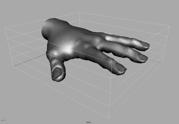
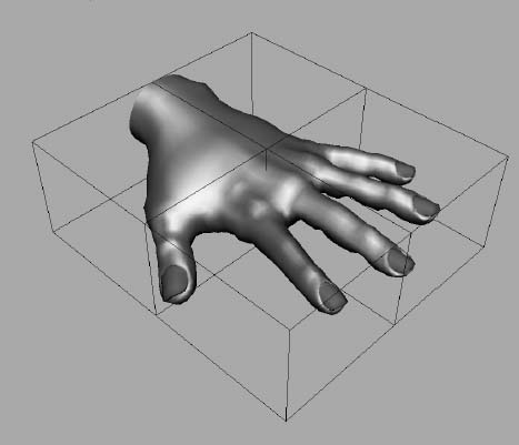
The alien hand in Figure 5.72 was created by adjusting the polygonal hand from this exercise using only lattices.

Figure 5.70 Position the lattice and its base to fit around the index finger.

Figure 5.71 Flare out the knuckles.

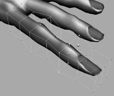
Figure 5.72 The human hand model is transformed into an alien hand by using lattices to deform the geometry.

As you can see, lattices give you powerful editing capabilities without the complication of dealing with surface points directly. Lattices can help you reshape an entire complex model quickly or adjust minor details on parts of a larger whole.

In Chapter 8, “Introduction to Animation,” you'll animate an object using another type of deformer. You'll also learn how to deform an object through a path.

Animating through a Lattice

Lattices don't only work on polygons; they can be used on any geometry in Maya and at any stage in your workflow to create or adjust models. You can also use lattices to create animated effects. In the next exercise, you'll animate an object through a simple lattice.

In the previous example, if you moved the hand geometry through the lattice while it was still applied to one of the fingers, you should have seen an interesting effect before you deleted the last of your lattices. The parts of the geometry of the hand deformed as the hand traveled through the lattice. Think of ways you can use this warping effect in an animation. For example, you can create the effect of a balloon squeezing through a pipe by animating the balloon geometry through a lattice.

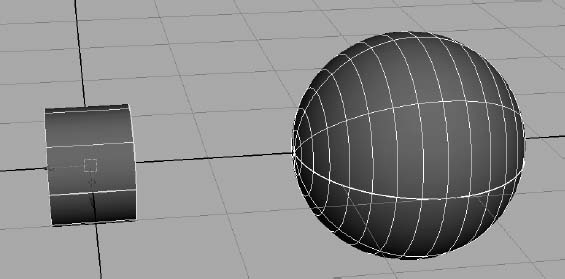
In the following exercise, you'll create a NURBS sphere with 8 sections and 16 spans, and an open-ended NURBS cylinder that has no end caps:

1. Choose Create NURBS Primitives Sphere , and set the Sections to 8 and Spans to 16 and create the sphere.
2. Choose Create NURBS Primitives Cylinder , and check None for the Caps option. Scale and arrange the sphere balloon and cylinder pipe as shown in Figure 5.73.

   Figure 5.73 Arrange the balloon and pipe.

   

3. Select the balloon, and create a lattice for it (see Figure 5.74). (From the Animation menu set, choose Create Deformers Lattice.) Set the S, T, and U Divisions to 4, 19, and 4, respectively. You set this number of lattice divisions to create a smoother deformation when the sphere goes through the pipe.
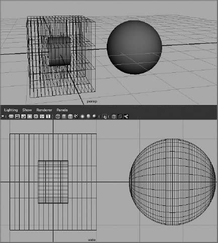
4. Select the lattice and its base in the Outliner (ffd1Lattice and ffd1Base nodes), and move the middle of the lattice so it fits over the length of the pipe (see Figure 5.75).

   Figure 5.74 Create a lattice for the sphere.

   

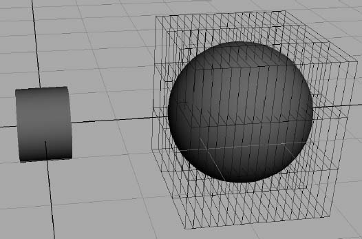
   Figure 5.75 Relocate the lattice to the cylinder.

   

5. Deselect the lattice base, and go to Component mode for the lattice. Select the appropriate points, and shape the lattice so the middle of the lattice fits into the cylinder (see Figure 5.76).

   Figure 5.76 Squeeze in the lattice points to fit the cylinder.

   

6. Select the sphere, and move it back and forth through the pipe and lattice. Notice how it squeezes to fit through. If you look closely, you'll see that the sphere starts to squeeze a little before it enters the pipe. You'll also see parts of the sphere sticking out of the very ends of the pipe. This effect, in which geometry passes through itself or another surface, is called interpenetration. You can avoid this by using a more highly segmented sphere and lattice. If you try this exercise with a lower-segmented sphere and/or lattice, you'll notice the interpenetrations even more. Figure 5.77 shows the balloon squeezing through the pipe.

In a similar fashion, you can create a lattice along a curve path and have an object travel through it. You'll try this in Chapter 8.

Figure 5.77 Squeezing the balloon through the pipe using a Lattice deformer

Subdivision Surfaces

Subdivision surfaces combine the best features of NURBS and polygonal modeling and are useful for intricate surfaces such as faces. Using subdivision surfaces, you can model complex characters and create models from single primitives (as in polygonal modeling) but with perfectly smooth surfaces (as in NURBS modeling).

Furthermore, with subdivision surfaces you have the added advantage that your surface won't tend to crease or tear at the seams as NURBS models made of patches of surfaces are prone to do. This leads to better models with which to animate organics.

Like lattices, subdivision surfaces rely on varying levels of editing detail that allow you to adjust a surface from a global level, where large parts of the model are modified, to a micro level, where you have control over the most dense surface points.

Typical subdivision workflow begins when you create a simple polygonal mesh of your model. The polygon is converted to a subdivision surface that you can edit using any number of subdivision detail levels. More often than not, the resulting subdivision surface is then converted back to a polygonal object for use in production. Subdivision surfaces can also be converted to NURBS patches.

The Subdivision surfaces (or SubDs, as they're called) toolset is found in the Surfaces menu set (press F4). You'll find yourself switching back and forth within the Polygons menu set (press F3). Just remember these hotkeys, and you'll be switching like a pro in no time.

Creating a Starfish

Now, you'll create a starfish model starting with polygons, like the models you created in Chapter 4. You'll then convert the polygon mesh to a subdivision surface to mold it into a proper starfish. Follow these steps:

1. Create a new scene, and switch into the Polygons menu set. With Interactive Creation turned off, create a polygon cube and scale it to be 8 wide, 8 deep, and 1.2 high.
2. Use the Split Polygon tool (Edit Mesh Split Polygon Tool) to split one side of the box into halves (see Figure 5.78). You can right-click every time you finish one of the splits without exiting the tool. When you do this, center the new edge by using the readout display in the Feedback bar (at the lower left of the screen) to place the split at 50 percent along each edge.

   When you invoke the Split Polygon tool, Maya's view panel prompts you to select along the first edge.

   

   Figure 5.78 Split the sides.

   

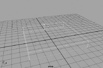
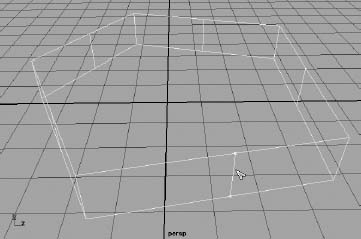
   Figure 5.79 After the pentagon is created, split each face into two.

3. Reshape the box into an irregular pentagon, as shown in Figure 5.79, by selecting the polygonal edges of the box in Component mode (F8) and moving them one by one. You needn't make all five sides exactly the same size—real starfish are irregular—but be careful not to move any of the edges up or down in the Y-axis because you want the pentagon to be flat.
4. Use the ever-popular Split Polygon tool again to cut all five sides in half, as shown in Figure 5.79. You'll use these edges to create a polygonal star, which you'll then convert to the subdivision surface.
5. Use the newly created edges to shape the pentagon into a star by moving the edges in toward the center (see Figure 5.80). This will be the basis for your starfish subdivision surface.
6. Save your work, and compare it to the scene file Starfish_v01.ma in the Starfish project from the companion web page.

Figure 5.80 Create a star shape.

Converting to a Subdivision Surface

Now that you have the basic polygonal shape for the starfish, convert it to a subdivision surface. Follow these steps:

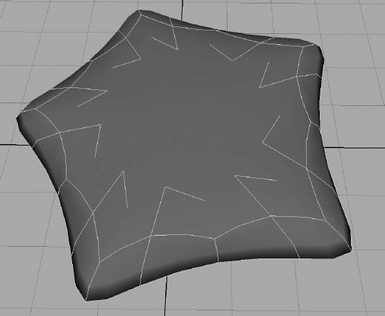
1. Select the star, and then choose Modify Convert Polygons To Subdiv. The star turns into a smooth subdivision surface, as shown in Figure 5.81.

   Figure 5.81 Converting the star shape to a subdivision

   

2. Although you've all but lost the points of the star by converting it to smooth subdivisions, you have far greater control. Press the 3 key to increase the display resolution of the surface. As they do with NURBS objects, the 1, 2, and 3 keys set the display resolution of a subdivision surface.
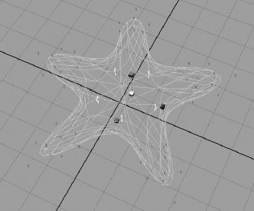
3. With the starfish still selected, switch to the Surfaces menu set (F4) and choose Subdiv Surfaces Polygon Proxy Mode. This switches Maya to a low-level editing mode and restores the shape of the star as a cage around the starfish (see Figure 5.82). Note that the star here isn't the surface of the starfish but a proxy that shapes the subdivision surface, much as a lattice does. Switch to Component mode (F8), and you see vertices on the polygon proxy (sometimes called a cage) that you can move to shape the starfish.
4. Change the display of the vertices of the subdivision surfaces before continuing. To do so, click Window Setting/Preferences Preferences and select Display Subdivs in the Categories list on the left. Set the Component display to Numbers for this exercise.
5. Using the polygon proxy to shape the starfish is a good way to create broad strokes when creating your final model. It won't yield good results by itself, however.

   Figure 5.82 The starfish's cage

   

   Press F8 to go back to the Object Selection mode, where you can select the starfish and not its vertices, and then switch back to Standard mode (choose Subdiv Surfaces Standard Mode). With the starfish still selected, enter Component mode to select vertices. The vertices of the starfish appear in the same locations as the points on the polygon proxy and are represented with zeros, as in Figure 5.83.

6. Right-click the starfish to open a marking menu, and choose Display Level 1. You'll define the arms of the fish at this level of detail. Select the vertices (now represented with 1s, as in Figure 5.84) between each point, and pull them in toward the center of the fish. This level of detail is automatically generated when you convert a poly image to a subdivision surface. Maya also has another level of detail (Display Level 2), which you'll use later.

   If by chance you don't see Display Level 2 as an option and Display Level 1 is the highest detail level you have, you can create a higher level of display by selecting all the level 1 vertices on the starfish in Component mode and choosing Subdiv Surfaces Refine Selected Components to create level 2 vertices. You'll then be able to choose Display Level 2 when needed.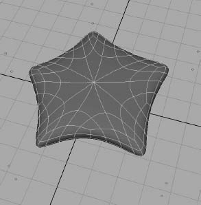

   

   Figure 5.83 The zeros represent the zero level of detail on this subdivision starfish and correspond to the vertices on its polygon proxy.

   

   Figure 5.84 Level 1 of the starfish

7. Save your file, and compare your work to the scene file Starfish_v02.ma in the Starfish project from the companion web page.
8. Right-click the starfish, and choose Display Level 2. The vertices on the next higher detail level appear and are represented by 2s. At this level of detail, you can move these vertices to give your starfish more character. Try making the areas between the points on the star smoother, as shown in Figure 5.85. Also try to flatten the bottom of the starfish using either level 1 or level 2 vertices.
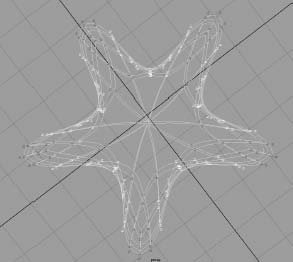
9. To achieve the appearance shown in Figure 5.85, you may need to detail your starfish further in some areas. As it stands now, the starfish can be edited up to level 2. To create another level of detail, select the areas you want to refine by selecting the level 2 vertices along the outside of each star point, as shown in Figure 5.86.
10. With those vertices selected, right-click the selection, and choose Refine Selected from the marking menu. Maya adds another level of detail to that area of the starfish with vertices marked as 2s. This allows you to make more detailed adjustments to the surface to mold it to your liking. Work the vertices at all levels to sculpt your starfish so it looks similar to the one in Figure 5.85.

    Right-clicking the starfish and choosing Refine Selected is the same as selecting the vertices and choosing Subdiv Surfaces Refine Selected Components. Choosing vertices in an area of your model and refining them beyond a display level of 2 creates more vertices for that area only. You can continue to refine your selection as needed. At any time, you can go back to Polygon Proxy mode to access the lowest level of detail and adjust the broad strokes of the model.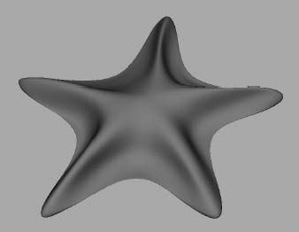

    

    Figure 5.85 A molded starfish

    

    Figure 5.86 Select the area to be refined.

11. Save your work again, and open the scene file Starfish_v03.ma in the Starfish project from the companion web page to compare your work with the model.

Building a Teakettle

Now that you've experienced the mechanics of subdivision surface modeling and editing, you're ready to tackle another model. The next subdivision exercise asks you to create a teakettle. You'll fashion the kettle from simple polygon shapes and then refine it using subdivisions.

Creating the Base Polygon Model

To create the base poly mesh for the kettle, follow these steps:

1. The main body of the kettle begins as a poly cylinder. Choose Create Polygon Primitives Cylinder to open the option box. Set Axis Divisions to 8, and set Height Divisions to 4.
2. To create the lid, create another poly cylinder with 8 subdivisions around the axis and 2 for the height. Scale it to fit as a lid on the first cylinder.
3. Select the upper row of poly edges on the lid, and scale them all in to create a bevel, as shown in Figure 5.87. Select every other edge on the top surface and delete them, as shown in Figure 5.88.
4. Select the poly edges of the main cylinder, and scale them out increasingly larger as you work your way down. Delete every other edge of the top surface as you did with the lid. Your kettle should look like the one in Figure 5.89.
5. Select the lid's top four faces. You can create a handle by extruding these faces and scaling them in. First, in the Polygons menu set, make sure the option Edit Mesh Keep Faces Together is enabled. This option lets you extrude these faces properly by keeping the poly faces together during the extrude operation. Now, select the four faces again, and choose Edit Mesh Extrude . Choose Edit Reset Settings to make sure the settings are correct, and click Extrude. Use the scale handles to scale the extruded faces in, as shown in Figure 5.90.

   If instead of following these directions you chose Edit Mesh Extrude and used the special scale handles shown in Figure 5.91, your faces may all separate.

6. With those four faces still selected, extrude the faces again, but this time pull them up and scale them in a bit, as shown in Figure 5.92.

   

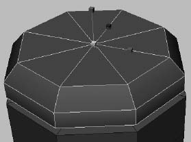
   Figure 5.87 Scale the outer edges inward.

   

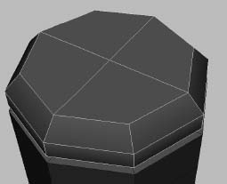
   Figure 5.88 Delete every other edge of the top surface.

   

   Figure 5.89 Creating the overall shape

   

   Figure 5.90 By default, faces extrude separately.

   

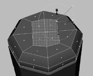
   Figure 5.91 The Keep Faces Together command allows you to extrude the faces together.

   

   Figure 5.92 Pulling up the lid's handle

7. Select the side faces of the lid's new handle, and extrude the faces inward using the scale handle to create detail on the handle.
8. Select the edges that make up the lid handle, and move them to round out the handle, as shown in Figure 5.93.
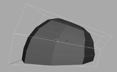
9. Select the four faces on the top of the kettle and extrude them. Scale the faces in and pull them up to round the top of the kettle, as shown in Figure 5.94.

   Figure 5.93 Round out the handle by moving the edges.

   

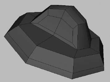
   Figure 5.94 Round off the top of the kettle.

   

10. Select the kettle, and apply a lattice to it by choosing Create Deformers Lattice (in the Animation menu set). In the Channel Box, with the new lattice select, set S Divisions to 2, T Divisions to 3, and U Divisions to 2. Adjust the lattice to bend the kettle back to create the front. Figure 5.95 shows the lattice's final position. When you have the proper shape, select the kettle and delete its History to delete the lattice.

    Figure 5.95 Use the lattice to bend the kettle.

    

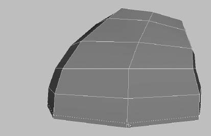
11. Just before you convert the kettle to a subdivision surface, you need to create more detail at the bottom of the kettle so the subdivision surface won't round out and you'll still have a flat bottom. In the Side or Front view panel, select the kettle. Go to the Polygons menu set (F3), choose Edit Mesh Insert Edge Loop Tool, and use the Insert Edge Loop tool to create a new division along the bottom of the kettle, as shown in Figure 5.96.

    Figure 5.96 Use the Insert Edge Loop tool to create a straight division line across the bottom.

    

12. Select all the new faces along the bottom and extrude them to create a lip that runs around the kettle's bottom, as shown in Figure 5.97. Be sure that Edit Mesh Keep Faces Together is still selected; otherwise, the faces will separate. Luckily, the Keep Faces Together option appears at the top of the Edit Mesh menu whenever you access the tools in that menu, so you can verify that it's enabled without too much bother.
13. Save your scene file, and load the Kettle_Model_v01.ma file from the Tea_Kettle project from the companion web page to compare your work up to this point.

Figure 5.97 Creating the base

Converting to Subdivisions

When you complete the base polygon model for the kettle, you can convert it to a subdivision surface to round it out and make it smooth. To convert the kettle, follow these steps:

1. Select the kettle, and choose Modify Convert Polygons To Subdiv. Select the lid and convert it as well.
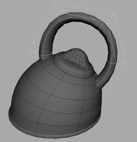
2. Select the converted kettle and the lid, and press 3 to view them in High-Resolution mode. Position the lid on top of the kettle. Your model should be similar to that in Figure 5.98.
3. The only items you still need to model are the spout and a handle. For the handle, create a subdivision torus (choose Create Subdiv Primitives Torus). Scale, rotate, and place the torus above and around the lid on top of the kettle.
4. With the handle selected, choose Subdiv Surfaces Polygon Proxy Mode in the Surfaces menu set. Using the vertices on the polygon proxy, make the handle thinner and elongate it upward, as shown in Figure 5.99.

   Figure 5.98 The subdivision kettle and lid

   

   Figure 5.99 The kettle's handle

   

5. Return to Standard mode with the handle selected (choose Subdiv Surfaces Standard Mode). To make the handle smoother, you can refine it and add more subdivisions. Switch to Component mode so the vertices of the handle display as 0s. Right-click the handle, and choose Refine Selected from the marking menu. New vertices appear as 1s. The handle should now be much smoother. Make any modeling adjustments to your liking. Using the right mouse button and the marking menu's Display Level command, switch between level 0 and level 1 displays as needed.
6. To create the spout, create a subdivision cylinder. Switch to Component mode to select the faces (not the vertices). Right-click the cylinder, and choose display level 2. Select the inside circle of faces on the top of the cylinder, as shown in Figure 5.100. Move them down into the cylinder to hollow it out, but create a thickness to the spout at the same time, as also shown in Figure 5.100.
7. Position the spout on the kettle. Move the vertices to flare out at the bottom of the spout where it meets the kettle. Figure 5.101 shows the completed kettle. Save your file.

Figure 5.100 Hollow out the spout.

Figure 5.101 The completed subdivision teakettle

Converting Back to Polygons

Most models created with subdivision surfaces should be converted back to polygons after the modeling is finished and rendering setup is ready to begin. Because subdivisions are a more intricate surface type than polygons, you'll probably have better performance while animating if you work with a polygonal model rather than a subdivision. Professionals frequently use subdivision tools and surfaces to create their models but then convert back to polygons after they're finished to avoid excessive memory usage while rendering.

This is a simple procedure, similar to the earlier exercise in which you converted NURBS surfaces to polygons. Here you'll convert the kettle back to polygons:

1. Select the subdivision kettle and its handle, spout, and lid, and choose Modify Convert Subdiv To Polygons to open the option box shown in Figure 5.102.

   Figure 5.102 The Convert Subdiv To Polygons option box

   

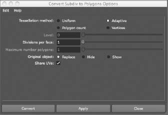
2. Select Adaptive for Tessellation Method. This option usually yields the best results.
3. The Divisions Per Face slider controls how smoothly the object is converted to polygons. For the best results, select each piece of the kettle separately and convert the pieces one by one, adjusting the Divisions Per Face value appropriately. A division value of 2 will work for everything but the handle, which requires a division value of at least 3 to remain fairly smooth.

More often than not, you'll want to take a model as far as possible before you convert it to polygons, but you should always save the original subdivision scene file in case it needs to be modified. This way, you can revert to your subdivision scene file, make your changes, and reconvert to polygons to render out the changes.

Taking the Kettle Further

Try creating more detail for the kettle or experimenting with your own designs. An easy addition is a whistle cap for the spout. You can also create a matching set of teacups and saucers with subdivision surfaces. With the skills you've acquired here, you should feel confident to tackle an entire kitchen full of models.

Summary

In this chapter, we tackled NURBS modeling by going through the usual surfacing tools, from lofting and revolving to bevels and boundary surfaces. Then, we explored the implications of surface History and how surfaces adjust to changes when History is enabled. You learned about different editing methods for NURBS surfaces, such as inserting isoparms and attaching surfaces together as well as converting those surfaces to poly meshes. You then put those lessons to work on creating a NURBS patch model for a steam pump for the locomotive model. Also in this chapter, we introduced you to the Artisan tool and how to use it to sculpt a NURBS surface.

This chapter covered various modeling techniques to help you break away from typical ways of thinking. You learned how to use a lattice to adjust a polygon hand model into an alien hand as well as how to animate a balloon pushing through a pipe. Moving on to a starfish model, you explored subdivision modeling techniques that are based on polygon modeling methods. Using polygons and SubDs hand in hand, you first made a teakettle out of polygons and then refined the model using subdivision modeling. Finally, you learned how to convert SubD models back to polygons.

As you've seen in this and in the previous chapter, and as you'll see in the next chapter, you can accomplish a modeling task in several ways. Different workflows give you the flexibility to choose your own modeling style. To make good choices, however, you'll need to practice. Good modelers have a strong eye for detail and a high tolerance for work that is repetitious. They also love assembling a complex object, and they're thrilled by the eventual outcome.

Keep at it; model everything you get your hands and eyes on. Try the same model a few different ways; switch between NURBS, polygons, and subdivisions to become comfortable with Maya's toolset. As you're doing that, stay on top of how you organize your nodes, and keep everything named and organized: the organization of your scenes is extremely important.

For further practice, use this chapter as a reference to create some of the following NURBS or subdivision models:

Bathroom Sink Snap a few digital stills of your bathroom sink, or find some pictures on the Internet. A sink will give you a great chance to explore NURBS surfacing, making pristine curves and smooth surfaces. It may be a bit involved, but it's not overwhelming.

Cartoon Head Use Maya Artisan and the Sculpt Geometry tool to turn an ordinary sphere into a cartoonish head. It's fun to use Sculpt Geometry to model. Try to make the head using only Artisan.

Human Hand Use the polygon model exercise in Chapter 4, but this time convert the base poly model you create to subdivisions and then add detail to it.

Computer Mouse A PC or Mac mouse makes a great simple SubD or NURBS model.