
Chapter 12
Particles and Dynamics
Animating large numbers of similar objects can be an arduous task to say the least. With hundreds, if not thousands, of individual objects and all of their animated parameters and transforms to consider, this is a task that, one object at a time, could quickly become overwhelming. Luckily, 3ds Max has several tools for animating large numbers of objects in a scene, including instanced objects, externally referencing objects, instanced modifiers, the Crowd utility for characters, and particle systems for controlling any number of particles. Particles are usually small objects, often in large numbers, that can represent rain, snow, a swarm of insects, a barrage of bullets, or anything else that requires a large quantity of objects that follow a similar action or are part of a larger system of movement.
Yet another method of creating simultaneous animations for several objects is through the use of reactor, the physics engine contained within 3ds Max. Using reactor, you can calculate the interactions between many rigid and soft body objects, or simulate fluids or rope dynamics.
Topics in this chapter include the following:
- Understanding particle systems
- Setting up a particle system
- Particle systems and space warps
- Using rigid body dynamics
- Using soft body dynamics
Understanding Particle Systems
Particle systems are a means to manage the infinite possibilities encountered when controlling thousands of seemingly random objects in a scene. The particles can follow a tight stream or emanate in all directions from the surface of an object, for example. The particles themselves can be pixel-sized elements on the screen or instanced geometry from an object in the scene. Particles can react to forces called space warps, such as wind and gravity, and bounce off objects called deflectors to give them a natural flow through a scene. Particles can even spawn new particles upon collision. There is a wide base of options when you are animating particle systems, especially when you are trying to simulate real-world effects such as smoke or rain.
All particle systems have two common yet distinct components: the emitter and the particles. The emitter, as the name suggests, is the object from which the particles originate. The location and, to a lesser extent, the orientation of the emitter are vital to the particles’ origination point in the scene. However, emitters are nonrendering objects, making their size and color unimportant.
Particles themselves are the elements that spew from the emitter. The number of particles can range from a few (to simulate a burst from a gun) to thousands (to simulate smoke from a burning building). As you would imagine, the number of particles visible in a viewport can adversely affect the viewport refresh speed and your ability to quickly navigate within the viewports. By default, far fewer particles are shown in the viewports than actually render in the scene. This helps maintain a reasonable system performance level.
Particle System Types
Two types of particle systems are available in 3ds Max: event-driven and non–event-driven.
Event-Driven Particle Systems
Event-driven particle systems use a series of tests and operators grouped into components called events. An operator affects the appearance and action of the individual particles and can, among many other abilities, change the shape or rotation of the particles, add a material or external force, or even delete the particles on a per-particle basis. Tests check for conditions such as a particle’s age, its speed, and whether it has collided with a deflector. Particles move down the list of operators and tests in an event and, if the particles pass the requirements of a test they encounter, they can leave the current event and move to the next. If they do not pass the test, the particles continue down the list in the current event. Particles that do not pass any test in an event commonly are deleted or recycled through the event until they do pass a test. Events are wired together in a flowchart style to clearly display the path, from event to event, that the particles follow.
Particle Flow is the event-driven particle system in 3ds Max, and it is a very comprehensive solution to most particle system requirements. The upper-left pane in the Particle View window in Figure 12-1 shows a partial layout of the events in a Particle Flow setup.
Figure 12-1: The Particle View window and a Particle Flow emitter

Events are green circles, operators are gray boxes, and tests appear as yellow diamonds. To the right of the Particle View window is a common example of one of the several emitter types that a Particle Flow can utilize. Using Particle Flow, you can create almost any particle-based effect, including rain, snow, mist, a flurry of arrows and spears, and objects assembling and disassembling in a blast of particles. Unfortunately, an in-depth examination of Particle Flow is beyond the scope of this book. However, we will familiarize you with the fundamentals of particles in the hopes you will be inspired to learn more in the course of your own work—which, when you think about it, is the best way to learn any program.
Non–Event-Driven Particle Systems
Non–event-driven particle systems rely on the parameters set in the Modify panel to control the appearance and content of the particles, as opposed to passing through events that may alter some of the particles. All particles are treated identically by the system’s parameters as a whole; there are no tests to modify the behavior for certain particles within the system. These particles can be bound to space warps to control apparent reactions to scene events, and they can be instructed to follow a path.
Non–event-driven particle systems have been around for a long time; they are stable, easy to learn, and an acceptable solution for many particle requirements. Non–event-driven particle systems are the focus of this chapter and will familiarize you with the workings of 3ds Max’s particle workflow.
Six different non–event-driven particle systems are available in 3ds Max; each has its own strengths.
- The SuperSpray particle system
- The Particle Array particle system
- The Particle Cloud particle system
- The Blizzard particle system
- The Spray particle system
- The Snow particle system
They all have similar setups and, after you understand one type, the others are easy to master.
The SuperSpray particle system is the most commonly used non–event-driven particle system in 3ds Max. It features a spherical emitter with a directional arrow to indicate the initial direction of the particles. It has eight rollouts containing the parameters that control the appearance and performance of the particles. The particles can emerge over a specified range of time or throughout the scene’s duration. When rendered, they can appear as one of several 2D or 3D shapes, as instanced scene geometry, or as interconnecting blobs that ebb and flow as they near each other. The particles can even spawn additional particles when they collide and load a predesigned series of parameters called a preset. The SuperSpray particle system essentially replaced the older, less-comprehensive Spray particle system, and it will be the main focus of this chapter. Figure 12-2 displays a SuperSpray particle system created in a viewport.
Rather than being the emitter, the Particle Array (also known as PArray) particle system, as shown in Figure 12-3, is only a visual link to the particle system emitter itself. The PArray uses an object in the scene as the emitter for the particles. While the parameters are adjusted with the PArray selected, the particles are emitted from the vertices, edges, or faces of the designated scene object. When used in conjunction with the PBomb space warp (discussed later in this chapter) and the Object Fragments setting, acceptable object explosions can be created.
Figure 12-2: The SuperSpray particle system

Figure 12-3: The Particle Array particle system

The Particle Cloud particle system, as shown in Figure 12-4, contains particles within a volume defined by the emitter or by selecting a 3D object in the scene to act as the constraining volume. When instanced geometry is used as the particle type, an array of space cruisers or a school of fish can be represented by the PCloud system. The PCloud object does not render, and any object used to constrain the particles can be hidden to give the illusion that the particles are not held in place by an external force.
Instanced geometry takes instanced copies of an object and assigns one instance to the particles in a scene. You can animate a school of fish, for example, by assigning an instanced fish model to particle locations and then animating the particles to school together and swim along.
The Blizzard particle system, which is similar to the SuperSpray particle system in its toolset and capabilities, is shown in Figure 12-5. The presets that ship with Blizzard are designed to simulate the particle motion of rain, snow, or mist. The Blizzard particle system has replaced the less-capable Snow particle system.
Figure 12-4: The Particle Cloud particle system

Figure 12-5: The Blizzard particle system

The Spray and Snow particle systems, shown in Figure 12-6, are the original particle systems that shipped with the initial release of 3D Studio Max, the first Windows release after four DOS-based versions of 3D Studio. At the time, they were cutting edge and beneficial, but they have not been improved significantly since their implementation. Spray and Snow do not offer primitive or instanced geometry as particles, presets, or particle spawning. The concepts used with these two systems are similar to the other more-advanced systems, but they are seldom used anymore.
Figure 12-6: The Spray and Snow particle systems

Particles are renderable objects in 3ds Max and are created in the Geometry tab of the Command panel. Like most other objects in 3ds Max, the particle system’s parameters can be changed immediately after they are created in the Create panel. Once you deselect the system, however, their parameters must be changed in the Modify panel, just like any other object in 3ds Max. To set up a particle system, follow these steps.
1. Click Create ⇒ Geometry ⇒ Particle Systems from the Command panel and then click on the SuperSpray button in the Object Type rollout. The particle system’s parameters appear in the Command panel (Figure 12-7).
Figure 12-7: The particle system’s parameters

2. Click and drag in the Perspective viewport to create the SuperSpray emitter. The emitters do not render, so the size does not matter; the arrow will point in the positive Z direction, as shown in Figure 12-8.
3. Drag the Time Slider to the right until the particles extend beyond the limits of the viewport. Frame number 10 should be sufficient. To see the mass of particles, click Zoom Extents to expand your Perspective viewport to show everything in the scene.
The Basic Parameters rollout controls how the particles spread as they exit the emitter, the size of the emitter, and how they display in the viewports.
4. In the Basic Parameters rollout, set both Spread values to 30 to spread the particles out 30 degrees in both the local X- and local Y-axes of the emitter. The Off Axis parameter rocks the emission direction along the X-axis and the Off Plane parameter rotates the angle of emission around the Z-axis. Both of these should remain at zero. See Figure 12-9.
5. In the Viewport Display area, make sure Ticks is selected and Percentage of Particles is set to 10. This ensures that the particles appear as small crosses in the viewports, regardless of the type of particle used, and that only 10 percent of the particles that are actually emitted are displayed in the viewport. Both of these parameters are used to ensure a minimal loss of performance in the viewport when particles are used.
6. Click the Render button (![]() ) in the Main toolbar. The particles appear as small dots in the Rendered Frame Window. If you cannot see them, try changing the object color in the Name and Color rollout in the Create panel of the Name field, and the color swatch in the Modify panel. In the next section, you will increase the size of the particles in the Rendered Frame Window by increasing the particle’s Size parameter. More particles are visible in the rendering than in the viewport because the Percentage of Particles value affects only the viewports and not the renderings.
) in the Main toolbar. The particles appear as small dots in the Rendered Frame Window. If you cannot see them, try changing the object color in the Name and Color rollout in the Create panel of the Name field, and the color swatch in the Modify panel. In the next section, you will increase the size of the particles in the Rendered Frame Window by increasing the particle’s Size parameter. More particles are visible in the rendering than in the viewport because the Percentage of Particles value affects only the viewports and not the renderings.
Figure 12-8: The SuperSpray emitter created in the Perspective viewport
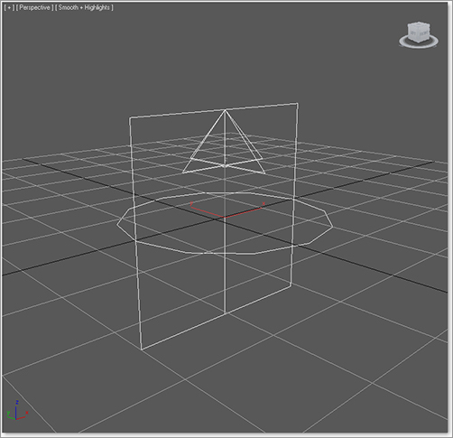
Figure 12-9: The Basic Parameters rollout

The Particle Generation Parameters
The parameters in the Particle Generation rollout control the emission of the particles, including the quantity, speed, size, and life span. If you can’t see any particles in your scene, the first place to look should be the Particle Generation rollout.
1. Expand the Particle Generation rollout (Figure 12-10).
Figure 12-10: The Particle Generation rollout
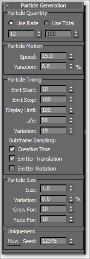
In the Particle Quantity area, the Use Rate value determines the number of particles emitted at each frame and the Use Total value determines how many particles are emitted over the active life of the system. Only one of these options can be active at a time. Increase the Use Rate value to 12.
2. Increase the Speed value to 15 to increase the velocity of the particles.
3. Below the viewports, next to the timeline, click the Play Animation button (![]() ). The particles spew from the emitter briefly and then stop. The particles have a distinct beginning and ending time that controls when the emitter can eject any particles.
). The particles spew from the emitter briefly and then stop. The particles have a distinct beginning and ending time that controls when the emitter can eject any particles.
4. In the Particle Timing section of the Particle Generation rollout, change the Emit Start value to 10, change the Emit Stop value to 100, and then click the Play Animation button again. The particle system will pause for 10 frames at the beginning of the active time segment and then emit 12 particles every frame for the remaining 90 frames.
5. Drag the Time Slider to frame 50 or so and then zoom out in the Perspective viewport until the limits of the particles’ extent are visible. Play the animation again. The particles increase their distance from the emitter until frame 40 and then travel no farther.
There are several parameters that determine when a particle is visible. The Emit Start and Emit Stop parameters mentioned earlier bracket the frames when the particles are emitted. The Display Until parameter in the Particle Timing area defines the last frame when any particle is visible. Regardless of whether this frame falls within the Start and Stop values, when the Display Until frame is reached, no more particles appear in the viewports or in any renderings. Another parameter that controls the display of particles is the Life value. The Life value determines how long each particle exists in a scene—from when it is emitted until it disappears. Currently, the Life value is set to 30 (as seen in Figure 12-10) so that at frame 40, which is 30 frames after the emission begins at frame 10, the particles disappear. Particles that are emitted after frame 10 also live for 30 frames, moving the same distance from the emitter before dying .
6. Change the Life value to 40, allowing the particles to travel one-third farther from the emitter, and change the Variation value, just below Life, to 20, adding randomness to the particle’s lifespan.
7. Play the animation. The particles now travel farther from the emitter and die between 34 and 48 frames after being emitted due to the Variation value we changed in step 6.
8. In the Particle Size area of the Particle Generation rollout, change the Size value to 10 and then render one frame of the scene at some point after frame 30. The result should look similar to Figure 12-11.
Figure 12-11: The SuperSpray particle system rendered in the Perspective viewport

Notice that the particles are smaller very near the emitter and also very far away from the emitter. By default, the Grow For value causes the particles to grow from a size of zero to full size over the first 10 frames of their lives. The Fade For parameter causes those same particles to shrink from full size to zero size during the last 10 frames of their lives.
9. Change the Fade For value to 0 so the particles retain their size at the end of their lives, and leave Grow For at its default.
10. Render the Perspective viewport again and notice how the particles grow, but never shrink. See Figure 12-12.
Figure 12-12: The particle system with the Fade For value changed to 0

Variation
In many situations utilizing particle systems, the particles are intended to appear as many similar but random objects. When the particles all have identical parameters (such as speed, life span, or rotation), the illusion of randomness disappears, which can greatly detract from its sense of reality. To alleviate this situation, in many of the parameter areas of the SuperSpray particle system’s rollouts, you will find a Variation parameter. The Variation settings modify their related parameters on a per-particle basis to add seeming randomness to the system. For example, changing the Variation parameter (below the Speed parameter) to 20 will assign a velocity to each particle within 20 percent of the Speed value. When the Speed parameter is set to 10 and Variation is set to 20, each particle is assigned to a random speed between 8 and 12—20 percent on either side of 10.
Putting It Together
Now that you have a basic understanding of particle systems, you will continue to work with them by creating a system that represents the bullets fired from a gun and the brass expelled from the ejection port. This will require two particle systems, one for each type of object leaving the gun. We will also examine the different particle types that can be emitted.
Creating the Particle Systems
The basic process of creating a particle system is fairly simple; you place the emitter in the scene, fine-tune its location and orientation, and then adjust the system’s parameters. The third item mentioned is the one that will take the most experimentation to perfect.
1. Open the Particle Gun.max file from the companion web page at www.sybex.com/go/intro3dsmax20011. This file is similar to the completed IK gun file created in Chapter 9, “Character Studio and IK Animation,” with a target, floor, materials, lights, and a camera added. The lights and camera have been hidden for clarity.
2. In the Top viewport, create a SuperSpray particle system. Move and rotate it so that the emitter is recessed slightly into the barrel of the gun, similar to Figure 12-13. Turn on the Angle Snap Toggle (![]() ) to rotate the system precisely 90 degrees.
) to rotate the system precisely 90 degrees.
Figure 12-13: The Top and Right viewports showing the proper placement of the SuperSpray particle emitter

3. Click the Select and Link button (![]() ) in the Main toolbar.
) in the Main toolbar.
4. Click and hold on the particle system; a rubber-banding line stretches from the emitter to the cursor. Place the cursor over the gun barrel and then release the mouse button. The gun flashes white to indicate that the linking is complete. Any changes in the gun’s orientation or position are now passed down to the particle system, keeping it co-located and oriented with the gun. See Figure 12-14.
Figure 12-14: Changes in the orientation or position are passed down to the particle system.

5. Rename this particle system SuperSpray Bullets.
6. Create a second SuperSpray particle system and place it on the right side of the gun body. Orient the emitter so that the particles are ejected upward and away from the gun, as shown in Figure 12-15.
7. Link this particle system to the gun, just as you did with the other in steps 3 and 4.
8. Rename this system SuperSpray Brass.
You may see a random particle or two already emitted by the particle systems. They are caused by the Emit Start time being set to the initial frame of the scene. This anomaly is corrected in the next section.
Figure 12-15: The Top and Front viewports showing the proper placement of the second SuperSpray particle emitter

Configuring the Particle System Timing
The number of particles emitted over time defines the density of the particles in the scene. The speed of the particles also factors into the proximity of the particles.
1. In the Time Controls area, click the Time Configuration button (![]() ).
).
2. In the Time Configuration dialog box, change the Length value to 300, as shown in Figure 12-16, and then click the OK button. At 30 frames per second (fps), the scene is now 10 seconds long.
3. Select SuperSpray Bullets and then click the Modify tab of the Command panel.
4. In the Particle Generation rollout, set the Use Rate to 10, the Speed to 10.0, the Emit Start value to 45, and the Emit Stop value to 300. After a one-and-a-half-second pause, the gun will fire then die off quickly.
5. Change the Display Until value to 300, as shown in Figure 12-17, so that the particles appear in the scene for the entire active time segment. Set the Life value to 300 so the particles do not die out in the scene.
Figure 12-16: The Time Configuration settings

Figure 12-17: Change the Display Until value to 300.

6. In the Particle Size section, change the Size value to 4. Drag the Time Slider to approximately frame 80 and then render the Camera viewport. The scene should look similar to Figure 12-18.
Figure 12-18: The rendered Camera viewport showing the particles

The particles appear as triangles that grow as they travel away from the emitter. When you are creating a traditional gun, this is not the look you want for the particles; the rounds should all appear the same size for the life of the particles. The particle type is covered in the next section and in the “Particle Systems and Space Warps” section later in this chapter. The conditions that allow the particles to pass through the Target object are also addressed.
Selecting the Particle Type
There are several types of particles that can be emitted by a particle system. Standard particles consist of eight different 2D and 3D particles, including cubes, spheres, and six-pointed stars.
The Facing Standard particle type is a square, 2D particle that maintains a continuous orientation perpendicular to the viewport. Using opacity mapped materials in conjunction with Facing particles can give the illusion of smoke or steam without using a massive number of particles. Facing particles are sometimes referred to as sprites.
MetaParticles use what is known as metaball technology, where each particle appears as a blob with a sphere of influence surrounding it. Whenever the two spheres of influence from two particles in close proximity overlap, the particles meld together in an organic manner similar to mercury or the wax in a lava lamp. Using MetaParticles can be computationally intensive, so caution should be a priority when that is the selected particle type. Start with a quantity of particles fewer than you would expect to use and then increase the amount, as required, after test rendering the scene.
Geometry that exists in the scene can also be substituted for the particles at render time. Using instanced geometry, a particle system can emit any objects from jet fighters to fire fighters, or nearly any other geometry in the scene, using the material from the object that is instanced. The original scene object can be hidden so as not to appear in the render of the scene, while still being instanced by the particle system.
To resume the Particle System exercise, continue with the following steps:
1. With the SuperSpray Bullets particle system selected, expand the Particle Type rollout.
2. In the Particle Types section, select MetaParticles.
3. From the menu bar, choose Edit ⇒ Hold to temporarily save the scene. If rendering the scene causes a system crash, it can be restored to this point using Edit ⇒ Fetch. 3ds Max is a stable program, but rendering MetaParticles can significantly task a computer system.
4. Render the scene. The particles that are near to each other combine to form blobs of meshes, as shown in Figure 12-19.
Figure 12-19: The rendered scene with the MetaParticles effect

5. In the MetaParticle Parameters section, decrease the Tension setting to 0.1. Tension controls a particle’s effort to maintain a spherical shape while in proximity to another particle. Lowering the Tension increases the amount of interparticle combining.
6. Render the scene again to see the effect of the lower Tension value, as shown in Figure 12-20.
Figure 12-20: The rendered scene with the lower Tension value

7. MetaParticles would be the solution if this gun were shooting out gobs of melted cheese, rather than working like a conventional machine gun. In this case, instanced geometry is the appropriate particle choice. Mmmmm, melted cheese.
8. Right-click on a blank area of the Active viewport and choose Unhide by Name from the Quad menu. Select the Bullet and Brass objects from the list in the Unhide Objects dialog box and then click the Unhide button. Two small objects, a bullet and a brass casing, appear below the gun.
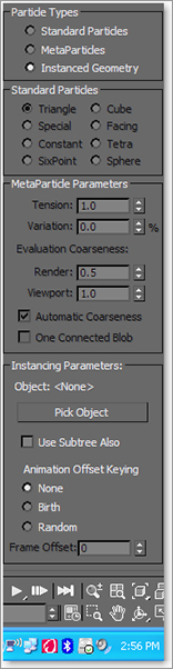
9. At the top of the Particle Type rollout, select Instanced Geometry for the particle type, as shown in Figure 12-21. In the Instancing Parameters section, click the Pick Object button.
Figure 12-21: The Particle Type parameters
10. Select the Bullet object in the scene. If necessary, press the H key to open the Pick Object dialog box to select the object by name. The bullet flashes white briefly to indicate that the selection is successful and the object name is now identified in the Instancing Parameters section as the instanced geometry object.
11. Render the Camera viewport. There are still a few problems that need to be corrected. The particles are growing as they leave the emitter, the particles grow to be too large for the gun barrel, and the bullets rotate on several axes rather than maintaining a forward orientation, as you can see in Figure 12-22. The bullets also display their object color, the color used by the particle system rather than the material applied to the Bullet object.
12. In the Particle Size section of the Particle Generation rollout, set the Grow For and Fade For parameters to 0. This will cause the particles to maintain a constant size throughout their life spans.
Figure 12-22: The rendered scene showing the large particles and rotating bullets

13. When using standard or MetaParticles, the Size parameter defines the size of the particle. When using instanced geometry, however, it becomes a multiplier of the object’s actual size. With the current Size value set to 4, the bullets are scaled to four times their modeled size. That’s a little big, so set the Size value to 1.
14. Expand the Rotation and Collision rollout. In the Spin Axis Controls section, select Direction of Travel/Mblur to make each bullet’s orientation follow its direction of travel, as shown in Figure 12-23.
15. At the bottom of the Particle Type rollout, make sure that the Instanced Geometry radio button is selected and then click the Get Material From button.
16. Render the Camera viewport again. All of the particles are now oriented properly, as you can see in Figure 12-24.
Figure 12-23: The Rotation and Collision settings

Figure 12-24: The rendered scene with all of the particles oriented properly

Setting Up the Other Particle System
We have a particle system set up to emit the bullets, and now we need one that ejects the brass casings from the machine gun. In many cases, the same parameters must be maintained among the two systems so these parameters will be wired together, ensuring a common value between them. This way the casings will shoot out with the bullets.
1. Continue with the previous exercise or open the Particle Gun1.max file from the companion web page.
2. Select the SuperSpray Brass particle system.
3. In the Particle Generation rollout, set the Size to 1 and set both the Grow For and Fade For values to 0. Set Emit Start to 45, Emit Stop to 300, Display Until to 300, and Life to 300.
4. In the Particle Motion section of the Particle Generation rollout, reduce the Speed value to 5. The rate of particles emitted is still set to 10; the Speed value just determines the velocity of the particles as they leave the emitter.
5. In the Particle Type rollout, choose Instanced Geometry in the Particle Types section and then click the Pick Object button. Select the Brass object as the geometry to be instanced.
6. Select the Instanced Geometry option in the Mat’l Mapping and Source section at the bottom of the Particle Type rollout, and then click the Get Material From button to define the material applied to the particles.
7. In the Rotation and Collision rollout, select the Direction of Travel/Mblur option.
8. Select the Bullet and Brass objects and hide them.
9. Drag the Time Slider, and your bullets and brass should emit together.
Wiring the Parameters Together
The values that define the parameters unique to each particle system in the scene have been set properly. Several values, such as the Use Rate, must maintain the same value for both particle systems so that, for example, the amount of brass ejected matches the number of bullets fired. These parameters can always be adjusted manually; however, the Parameter Wiring tool forces one object’s parameters to drive another’s. In the following exercise, the parameter values of the SuperSpray Bullets particle system are used to define the parameter values of the SuperSpray Brass particle system. By wiring parameters together, you can control more than one system by manipulating only one of them.
1. Continue with the previous exercise or load the Particle Gun2.max file from the companion web page.
2. Select the SuperSpray Bullets particle system. Right-click in the viewport and choose Wire Parameters from the Quad menu. See Figure 12-25.
Figure 12-25: Choose Wire Parameters from the Quad menu.

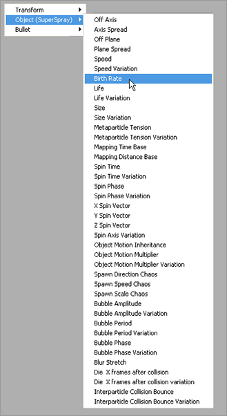
3. From the small pop-up menu that appears, choose Object (SuperSpray) and then Birth Rate from the cascading menu (Figure 12-26). A rubber-banding line connects the particle system to the cursor. At this point, the object to be wired to the SuperSpray Bullet’s Birth Rate parameter must be selected.
4. Press the H key to open the Pick Object dialog box, select SuperSpray Brass (Figure 12-27), and then click the Pick button.
5. From the small pop-up menu that appears, choose Object (SuperSpray) and then Birth Rate from the cascading menu (Figure 12-28).
6. The Parameter Wiring dialog box opens, as shown in Figure 12-29. The Birth Rate parameters are highlighted in both the left and right windows. The left side of the dialog box displays the SuperSpray Bullets particle system’s parameter, and the right side displays the SuperSpray Brass particle system’s parameter.
7. The control direction, defining which parameter controls the other, can be set so that either one of the parameters controls the other, or bidirectional control can be set so that either parameter can change the other. In this case, the bullet rate is used to control the brass rate. Click the right arrow between the two parameter windows, as shown in Figure 12-30.
Figure 12-26: Wire the selected object to the SuperSpray Bullet’s Birth Rate parameter.

Figure 12-27: Select SuperSpray Brass in the Pick Object dialog box.

Figure 12-28: Select Object (SuperSpray) and then Birth Rate.
8. Complete the wiring process by clicking the Connect button. The parameters in each window will turn a color to indicate that they are wired.
9. Select the SuperSpray Bullets particle system and change the Use Rate setting to 12.
Figure 12-29: The Parameter Wiring dialog box with the Birth Rate parameters highlighted

Figure 12-30: Click the right arrow between the two parameter windows.

10. Select the SuperSpray Brass particle system and examine its Use Rate. It is now set to 12 as well.
You can try to change the Use Rate for the SuperSpray Brass particle system, but it won’t be effective. The related spinners simply do not work, and they shouldn’t because the particle system’s Use Rate is defined by the Use Rate of the SuperSpray Bullets particle system. You can highlight and change the value manually; however, nothing will really happen. When you deselect the system and then select it again, the Use Rate reverts to the value set by the other system.
11. Select the Life parameter in both windows; click the right arrow and then the Connect button. The Life parameters are now wired together as well.
Unfortunately, the Emit Start, Emit Stop, and Display Until parameters are not exposed to the Parameter Wiring dialog box. These values must be changed for each particle system manually.
12. Close the Parameter Wiring dialog box.
13. Drag the Time Slider. The two particle systems emit equal numbers of particles at the same time. The brass ejects in a straight line from the gun body, as shown in Figure 12-31. The straight-line emission is corrected in the next section. You can now change the rate at which the bullets fire, and the brass will eject properly automatically!
The particle systems have been created and linked to the gun so that they maintain the proper position and orientation when the gun moves or rotates. The systems have been adjusted to fire bullets from the barrel and eject brass from the side at an equal and wired rate. The next section covers the processes of adding space warps to interject gravity into the scene and to cause the particles to collide with scene objects.
Figure 12-31: The straight-line emission

Particle Systems and Space Warps
Space warps are nonrendering objects that can modify or manipulate the objects in a scene. Modifier-based space warps, for example, deform objects based on the object’s proximity to the space warp. In this section, the focus is on the Forces and Deflectors categories of space warps, the space warps that affect particle systems.
The Forces space warps affect particle systems by altering the trajectory of the particles as they move through the scene. Each space warp displays as an icon in the viewports that must be bound to each object that it is designated to affect. The bindings appear as wide gray lines at the top of the Modifier Stack.
The Forces space warps are listed here:
Motor Applies a directional spin to the particles, creating a circular movement. The orientation of the Space Warp icon defines the direction of the rotation.
Vortex Similar to the Motor space warp, Vortex causes the particles to move in a circular motion but also decreases the radius of the motion over distance, creating a funnel-shaped motion.
Path Follow Requires the particles to follow a spline path. The particle timing is controlled by the Path Follow’s parameters.
Displace Changes the particle trajectory by pushing them based on the space warp’s Strength and Decay values. Image maps can also be used to define the amount of displacement.
Wind Adds a directional force to the particles based on the space warp’s orientation. Randomness can be added to increase the realism of the simulation.
Push Applies a constant, directional force to the particles.
Drag Rather than changing the direction of the particles, Drag slows the speed of the particles as they pass through its influence.
PBomb Disperses particles with a linear or spherical force. This can be effective when used with the Particle Array particle system.
Gravity Applies a constant acceleration used to simulate the effect of gravity on the particles. Gravity can be applied in a linear fashion.
Adding Gravity to a Scene
When looking at the particle systems in the previous exercises, especially the SuperSpray Brass system in our machine gun scene, it’s evident that the motion of the particles is not realistic. The particles are emitted at approximately a 45-degree angle up and away from the gun body. The particles maintain a perfectly straight trajectory and never fall to the earth as they should. In this exercise, gravity is added to both particle systems to cause the bullets and brass to drop. To begin the exercise, follow these steps:
1. Continue with the previous exercise or load the Particle Gun3.max file from the companion web page.
2. Drag the Time Slider to frame 100.
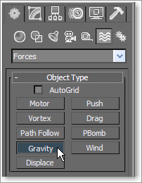
3. Click Create ⇒ Space Warps. Choose Forces from the drop-down menu if necessary, and then click the Gravity button (Figure 12-32).
Figure 12-32: The Gravity Button in Space Warps
4. Click and drag in the Top viewport to place and size the Gravity Space Warp icon. The size and the location are unimportant, but the orientation of the icon defines the direction of the gravitational force. See Figure 12-33.
5. Select the SuperSpray Brass particle system. Click the Bind to Space Warp button (![]() ) in the Main toolbar.
) in the Main toolbar.
6. Click on the Particle System emitter or the particles themselves and drag the cursor toward the Gravity Space Warp icon. A rubber-banding line connects the particle system to the cursor.
7. Place the cursor over the Gravity space warp; when the cursor’s appearance changes to identify it as a valid object for binding, release the mouse button. The space warp flashes briefly to indicate a successful binding, and the particles drop through the floor as shown in Figure 12-34.
8. Select the SuperSpray Bullets space warp and bind it to the Gravity space warp as well.
9. Play the animation. The particles from both systems are affected by the gravity, but the bullets drop too far for their distance from the gun to the target. Reducing the amount of gravity isn’t appropriate because the brass would fall too slowly and the gravitational force should be consistent throughout the scene. This situation is fixed by increasing the velocity of the bullets as they leave the barrel.
Figure 12-33: Click and drag in the Top viewport to place and size the Gravity Space Warp icon.

Figure 12-34: After the particle system is bound to the Gravity space warp, the particles drop through the floor.

10. The Bind to Space Warp button is still active. Click the Select Object button, and then select the SuperSpray Bullets particle system.
11. Make sure the Time Slider is at a frame well into the animation so that changes to the system are reflected in the viewports.
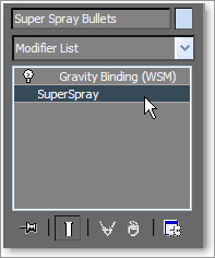
12. In the Modify panel, click the SuperSpray entry in the Modifier Stack (Figure 12-35) to expose the particle system’s parameters.
Figure 12-35: Click SuperSpray in the Modifer Stack.
13. In the Particle Generation rollout, increase the Speed value to 50. The visible trajectories of the particles will flatten out.
At the bottom of the Rotation and Collision rollout, you will find the Interparticle Collisions section. Enabling this parameter causes 3ds Max to calculate and determine the result of any situation where two particles impact each other. This can add a measure of realism to the way the particles react, but it can also consume a significant amount of system resources. Use this feature with caution and always perform an Edit ⇒ Hold on the scene prior to enabling or testing the feature.
Controlling the Particles with Deflectors
As you saw in the previous exercises, particles travel through a scene, guided by space warps but unaffected by geometry. Deflectors are a type of space warp that causes the particles that impact the deflectors to bounce as if they have collided with an immovable surface. The amount of bounce assigned to a deflector is a multiplier that defines the velocity of a particle after it impacts the space warp. A Bounce value of 0.5 results in the particle’s speed being reduced to 50 percent of the speed it had when it hit the deflector. Most deflectors have Time On and Time Off parameters that control when the deflector is active.
Deflecting the Brass at the Floor
To get the spent casings to collide with the ground, follow these steps:
1. Continue with the previous exercise or load the Particle Gun4.max file from the companion web page.
2. Drag the Time Slider to frame 100.
3. Click Create ⇒ Space Warps. Choose Deflectors from the drop-down menu and then click the POmniFlect button (Figure 12-36).
Figure 12-36: The POmniFlect button for the Deflectors pull-down option

4. In the Top viewport, click and drag to define the two opposite corners of the deflector. The deflector should be similar in size to the Floor object in the scene. Unlike the Forces space warps, deflectors must be positioned in the stream of the particles, as shown in Figure 12-37.
5. Move the deflector 0.3 units in the positive Z direction. The impact point is based on the particle location. When using instanced geometry, the particle location is defined by the center point of the geometry. The bullets and brass are about 0.3 units in radius, so moving the deflector up 0.3 units prevents the particles from sinking into the floor.
6. Select the SuperSpray Brass particle system and then click the Bind to Space Warp button in the Main toolbar. Click on the particle system, or particles, drag to the perimeter of the deflector, and then release to bind the deflector to the particle system.
7. Activate the Camera viewport and then play the animation. The particles initially bounce equal in height to their highest point after being ejected, but they discontinue shortly afterward.
8. Select the Deflector object in the viewport, not the deflector binding in the Modifier Stack.
Figure 12-37: The deflector must be positioned in the stream of the particles.

Understanding Deflector Names
The names assigned to the different deflectors distinguish the shapes and properties of those deflectors. Understanding the deflector naming convention is key to selecting the correct deflector for the task at hand.
- If the deflector name begins with a P or an S, the deflector is Planar or Spherical, respectively.
- If the deflector name begins with a U, this is a universal deflector and any scene geometry can be assigned as a deflector, instead of the Deflector icon itself.
- If the deflector name ends with “OmniFlect,” this deflector affects all particles that impact it. The OmniFlect deflectors are more advanced than the simpler space warps that end with “Deflector.”
- If the deflector name ends with “DynaFlect,” this deflector affects all particles that impact it and, when used with dynamic simulations, can affect other objects in the scene.
9. In the Timing section of the Parameters rollout, set the Time Off value to 300, as shown in Figure 12-38, to leave the deflector on during the entire active time segment.
Figure 12-38: POmniFlect parameters

10. In the Reflection section, set the Bounce value to 0.25 and the Variation value to 10 percent. Increase Chaos to 50 percent so the particles’ directions are not constrained to a straight line.
11. In the Common section, increase the Friction value to 4.0 to prevent the particles from spreading too far along the deflector’s surface, as shown in Figure 12-38.
12. Play the animation. The brass is ejected from the side of the gun, falls to the floor, and spreads a bit from the point of impact.
Deflecting the Bullets at the Target
The brass is handled, and now the bullet collisions need to be addressed.
1. Click Create ⇒ Space Warps, and then click the UOmniFlect button.
2. In the Top viewport, click and drag to place and size the universal deflector. The size and position do not matter. This is just a visible icon. A scene object will be selected to act as the deflector. See Figure 12-39.
3. Select the SuperSpray Bullets particle system, and bind it to the UOmniflect icon, not the Target object. Bind the particle system to the POmniFlect deflector as well.
4. Click the Select Object button and then select the UOmniFlect icon.
5. In the Modify panel, click the Pick Object button and then select the Target object in the scene.
6. In the Timing section, set the Time Off value to 300.
7. In the Reflection section, set Bounce to 0.01, Variation to 10, and Chaos to 4.
8. Play the animation. The particles hit the target, fall to the floor, and then spread out a bit.
As you can see, the proper use of Force and Deflector space warps, in conjunction with particle systems, can successfully animate thousands of small objects within the constraints of a scene. The completed scene can be examined using the Particle Gun Complete.max and Particle Gun.avi files on the companion web page. In the remaining sections in this chapter, we will look at the implementation of rigid and soft body dynamics in physics simulations.
Figure 12-39: In the Top viewport, click and drag to place and size the universal deflector.

Part of the core package of 3ds Max is the physics engine known as reactor. With reactor, complex physical conditions are accurately animated showing the interaction of the scene objects with each other and with external forces such as wind or gravity. Objects are assigned mass, elasticity, and friction properties, and designated as movable or immovable objects. Rigid body dynamics, soft body dynamics, rope, and cloth simulations are all within the limits of reactor’s toolset. The Real Time Preview window displays a lower-resolution, unrendered example of the animation to be created to make it easy to visualize how your dynamic simulation will run, without a lot of wait. The reactor engine calculates the animation, but the standard practice of creating keyframes is the final output of the simulations. These keyframes can be edited and manipulated; however, the integrity of the simulation could be compromised.
Creating the Simulation Objects
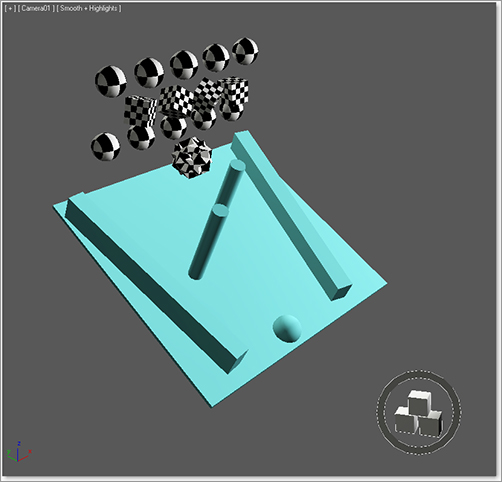
In this exercise, a series of primitive objects is dropped onto a complex inclined object to examine the interaction of the scene objects, as shown in Figure 12-40. Although this is a simple example of the use of the physics simulator, reactor can be used to simulate the interactions of very complex scenes with many colliding objects and external forces.
Figure 12-40: A series of primitive objects is to be dropped onto this complex inclined object.

1. Open the Rigid.max file from the companion web page. This consists of an inclined box with additional boxes, cylinders, and a hemisphere placed on its surface to make the simulation more complex.
2. Create two rows of spheres above the inclined board. Make sure they are all over the top edge of the board and fit between the two angled rails on the sides.
3. Create a row of small boxes between the rows of spheres as shown, and rotate them each about all three axes to offset them.
4. From the Extended Primitives category of geometry objects, create a Hedra, then go to family group and choose Star 2 and position it near the other objects. The scene should look similar to Figure 12-41.
5. Open the Material Editor and then apply the Checker material to all of the objects you created. The Checker Diffuse Color map helps discern the rotation of each object in the simulation.
Figure 12-41: The scene after creating additional objects for the simulation

Assigning the Physical Properties
Each object in the scene must be assigned the correct properties to define their reactions during the simulation. Note that any objects that are to be stable and immovable are assigned a Mass value of 0.
Figure 12-42: Open the Rigid Body Properties dialog box.
1. Select all of the objects that make up the inclined board in the scene.
2. Right-click an empty area of the Main toolbar to display a list of available toolbars, then choose reactor. This will bring up the floating toolbar. Right-click on the title bar and choose Dock ⇒ Left.
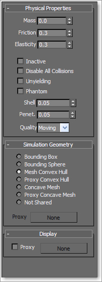
3. From the reactor toolbar, click the Open Property Editor button (![]() ) to open the Rigid Body Properties dialog box shown in Figure 12-42.
) to open the Rigid Body Properties dialog box shown in Figure 12-42.
4. Make sure Mass is set to 0 in the Physical Properties rollout, and Mesh Convex Hull is selected in the Simulation Geometry rollout.
5. Select all of the spheres that you created. Set their Mass value to 1.0 and choose Bounding Sphere in the Simulation Geometry rollout, as shown in Figure 12-43. When using a spherical object, Bounding Sphere is more accurate and calculates faster than Mesh Convex Hull.
Figure 12-43: Choose Bounding Sphere in the Simulation Geometry rollout.

Most 3D geometry works as expected during a reactor simulation. However, reactor contains its own Plane object for use whenever flat, 2D surfaces are required. When a 3ds Max plane is used instead of a reactor plane, Concave Mesh must be chosen as the Simulation Geometry type.
6. Select all of the boxes that you created, assign a Mass value of 1.0, and choose the Bounding Box option.
7. Select the hedra. Increase its mass to 1.0 and select Mesh Convex Hull for the simulation.
You have now assigned dynamic parameters to the scene objects; however, there is more to do to set up the simulation.
The Simulation Geometry Rollout
The Simulation Geometry rollout defines how reactor defines the surfaces of an object during the simulation.
- The Bounding Box and Bounding Sphere options place the extents of the objects, as far as the simulation is concerned, at the limits of the smallest possible box or sphere that could encompass them.
- Mesh Convex Hull closely follows the extents of the object, with all vertices included within the simulation volume, while spanning any concave areas. Complicated meshes can increase the calculation time when using Mesh Convex Hull, so the Proxy Convex Hull option allows a less dense substitution object to be used to define the simulation parameters.
- When Concave Mesh is used, the actual surface of the geometry is used. This can drastically increase the calculation time and should be used only when necessary. Using the Proxy Concave Mesh option can reduce the simulation time when using a complicated object.
- 3ds Max assigns the Not Shared option to the selected geometry when multiple objects are selected that do not utilize the same Simulation Geometry setting.
Creating the Collection
Scene objects must be members of a collection to be included in any simulations. The collections appear as simple icons in the viewports that are selected to access the simulation’s parameters, including editing the list of included objects.
1. Continue with the previous exercise or open the Rigid1.max file from the companion web page.
2. Click the Create Rigid Body Collection button (![]() ) in the reactor toolbar.
) in the reactor toolbar.
3. Click in any viewport to place the Rigid Body Collection icon, as shown in Figure 12-44. The location does not matter.
Figure 12-44: Click in any viewport to place the Rigid Body Collection icon.
4. In the Command panel, click the Add button at the bottom of the RB Collection Properties rollout (Figure 12-45).
Figure 12-45: Click the Add button in the RB Collection Properties rollout.

Figure 12-46: The Select Rigid Bodies dialog box

5. In the Select Rigid Bodies dialog box that opens, select all of the objects in the scene except for the collection itself and then click the Select button; see Figure 12-46. The object names will appear in the Rigid Bodies field in the Command panel.
In most cases, not every object in a scene is required to be in a simulation. An object should be omitted if its impact on the simulation is not required. For example, in a scene where marbles spill across a table and onto a floor, the marbles, table, and floor must be included, but the nearby lamp or the ceiling should be omitted.
Testing the Simulation
The reactor engine provides the Real-Time Preview window where you can view the simulation. Materials and lighting are not considered for this preview; therefore, it is much faster, but less accurate, than rendering the animation.
1. Click the Preview Animation button (![]() ) in the reactor toolbar. The reactor engine analyzes the simulation and then opens the reactor Real-Time Preview window shown in Figure 12-47.
) in the reactor toolbar. The reactor engine analyzes the simulation and then opens the reactor Real-Time Preview window shown in Figure 12-47.
Figure 12-47: The reactor Real-Time Preview window showing the scene
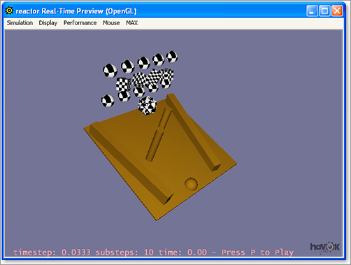
2. Press the P key to begin the preview, and then press P again to stop it.
3. After the preview runs its course, choose Simulation ⇒ Reset to place the objects at their starting points and review the animation.
You can click and drag in the Preview window to orbit around the simulation objects.
4. The hedra is large for the scene and may cause a bottleneck. Close the Preview window.
5. Select the hedra and reduce its Radius value.
6. Select all of the objects of the inclined board, and then open the Rigid Body Properties dialog box as shown in Figure 12-48.
Figure 12-48: The Change Friction property in the Rigid Body Properties dialog box

7. Set the Friction property to 0.1.
8. Select the remaining objects in the scene, and set the Friction to 0.1 as well.
9. Rearrange the objects to change the simulation to your liking.
10. Continue to preview the animation and rearrange the objects until the simulation meets your liking.
Creating the Animation
The Preview window showed what the animation will be like, but the animation keys have not been created from the simulation. The next exercise creates keys for all the objects in the collection. Creating the keys is not undoable, so it is recommended that an Edit ⇒ Hold be performed prior to creating the animation. This will create a return point in the scene in case something goes awry. This way, you can use Edit ⇒ Fetch to come back to this place in your workflow.
1. In the Time Configuration dialog box, increase the length of the scene’s animation to 200 frames then click OK.
2. Click Edit ⇒ Hold from the Main menu.
Figure 12-49: The reactor dialog

3. Click the Create Animation button (![]() ) from the reactor toolbar.
) from the reactor toolbar.
4. Click OK in the reactor dialog box that opens and warns you that the action cannot be undone, as shown in Figure 12-49.
3ds Max creates keys at every frame for every object in the simulation. The process of creating keys with reactor cannot be undone, but the objects can be selected and their keys can be deleted in the track bar, the Dope Sheet, or the Function Curve dialog boxes.
5. Play the animation. The scene animates through frame 100 and then stops. The default value for all simulations is 100 frames.
6. To restore the scene to its state before 3ds Max created the animation, click Edit ⇒ Fetch from the Main menu and then click the Yes button in the dialog box that opens.
7. Click the Utilities tab (![]() ) of the Command panel.
) of the Command panel.
8. Click the reactor button in the Utilities rollout.
In reactor, solvers provide the algorithms that determine each object’s reactions in the simulation. The two available solver options in 3ds Max 2011 are Havok 1 and Havok 3. The Havok 1 solver has more functionality and can handle all types of simulation objects. Havok 3 is faster and more accurate, but it can solve only for rigid body objects. If only rigid body objects are used in a simulation, Havok 3 is usually the better choice.
9. In the About rollout, select Havok 3 from the Choose Solver drop-down menu. Havok 3 is the better choice when using only rigid body objects.
10. Expand the Preview & Animation rollout and change the End Frame value to 200.
11. Click Edit ⇒ Hold again, and then click the Create Animation button shown in Figure 12-50.
Figure 12-50: Click the Create Animation button.

12. 3ds Max creates keys based on the simulation. You can fetch the scene and rearrange the objects as you want to change the simulation parameters and rerun the animation. Remember to hold the scene before creating the animation each time, so you can easily go back to your hold point.
The completed exercise is available as the Rigid Complete.max file in the Dynamics Scene Files folder on the companion web page and the final rendering as Rigid Complete.avi.
Soft body objects differ from rigid body objects in that they can deform upon impact with other objects in the scene. To be included in a simulation as soft body objects, scene objects must have the Soft Body modifier applied and be members of a soft body collection. Soft body objects can interact with rigid body objects in the same simulation. Physical properties are assigned to soft body objects in the same manner that they are assigned to their rigid counterparts.
Creating the Collections
Before you can simulate the reactions between soft body objects, all objects considered in the simulation must be contained in a collection.
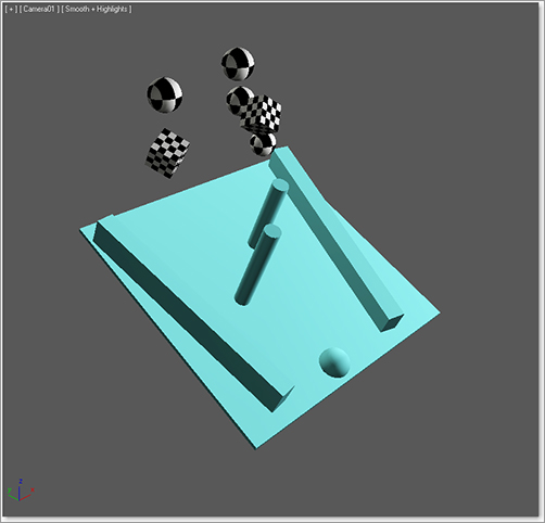
1. Open the Soft.max file from the Dynamics Scene Files folder on the companion web page. As you can see in Figure 12-51, this is a simpler version of the project used in the previous exercises.
Figure 12-51: This is a simpler version of the project.
2. Select all of the base objects, and then click the Create Rigid Body Collection button in the reactor toolbar. The icon is placed at the center of the selection, and the selected objects are added to the collection.
3. Select the spheres and boxes with the Checker material applied.
4. Click the Apply Soft Body Modifier button (![]() ) in the reactor toolbar.
) in the reactor toolbar.
5. With the objects still selected, click the Create Soft Body Collection button (![]() ) in the reactor toolbar. The falling objects are automatically added to the soft body collection.
) in the reactor toolbar. The falling objects are automatically added to the soft body collection.
6. Move the Collection icons away from the scene geometry. Your Perspective viewport should look similar to Figure 12-52.
Figure 12-52: The Perspective viewport with the rigid- and soft-body collections

Creating the Animation
In the earlier exercise, the Havok 3 solver was selected because of its capabilities when using rigid body objects exclusively. With the combination of both soft and rigid objects in this exercise, the Havok 1 solver is the better choice.
1. In the Utilities panel, click the reactor button and then choose Havok 1 from the drop-down menu in the About rollout, as shown in Figure 12-53.
Figure 12-53: Select the Havok 1 solver.

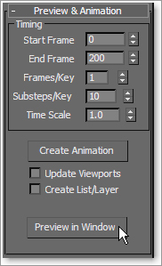
2. Click the Preview Animation button in reactor and play the animation in the reactor Real-Time Preview window, shown in Figure 12-54. The animation plays slower than the rigid body preview due to the more complex animation required by the deforming meshes.
Figure 12-54: Click the Preview in Window button.
In a complex scene, or on a slow computer, the reactor Real-Time Preview may display the scene at a rate that is too slow to easily determine the effectiveness of the simulation. In these cases, you need to create the animation and then, if revisions are required, delete all of the simulation objects’ animation keys before making any changes and re-creating the animation.
3. Close the Preview window.
4. The parameters of individual objects can be set in the reactor SoftBody modifier’s settings. Select one of the spheres and then, in the Modify panel, change its Mass to 2, Stiffness to 4 and Friction to 0.1. Repeat this step with one more sphere and one of the boxes. The larger Mass value will cause the object to impact with a greater force.
5. Test the animation again. Continue to make changes and then, when you are satisfied, hold the scene.
6. Click the Create Animation button in the reactor toolbar to create the animation using the properties assigned to the objects.
The completed exercise can be found on the companion web page as Soft Complete.max and Soft Compete.avi.
This chapter introduced you to both Max’s non–event-driven particle systems and the reactor physics simulation engine. Using particles, thousands of seemingly random or purposeful objects can be animated by effectively manipulating the particle system’s parameters. Particles can appear as primitive shapes, interconnecting blobs, or any instanced geometry object from the scene. Particle systems can be affected by external forces, such as gravity, wind, or vortex, and they can bounce off many types of deflectors positioned within the flow of particles.
The reactor component of Max is a powerful tool for creating accurate animations based on the interactions of scene objects. Rigid or soft body objects in collections can impact each other and deform, bounce, or slide away based on the objects’ physical properties. Animations can be previewed and then thousands of animation keys can be created quickly to fulfill a scene’s physics-based animation requirements.
So Long, and Thanks for All the Fish
And that’s about it for us. (Awkward pause. Do you lean in for a hug, or go for a simple handshake?) We hope you found this text illuminating and helpful in priming you for a fruitful and exciting education in Autodesk’s 3ds Max. There are so many resources to be found in bookstores and on the Internet that you should feel confident and secure in jumping into the next step of your CG education.
By now, you should be familiar with the workings of 3ds Max and know what parts of the CG process you find appealing. Whether it’s modeling or lighting, animating or dynamics, you now have a firm grasp of how to get things done. If you feel shaky in some areas, we strongly recommend going back to the related chapters and redoing the exercises to build your confidence.
We hope the most important idea you take with you from this book is the notion that proficiency in and mastery of a CG program such as 3ds Max takes patience and practice. The best way to learn is to experience the software in pursuit of your own artistic endeavors. Don’t be afraid to throw yourself into your own personal projects, challenging yourself to get better with every effort. Treat this text as a formal introduction to all that 3ds Max has to offer your artistic work, and forge ahead. Have fun, and good luck!