
Chapter 7
Materials and Mapping
Applying materials is the phrase used in 3ds Max to describe applying colors and textures to an object. A material defines an object’s look—its color, tactile texture, transparency, luminescence, glow, and so on. Mapping is the term used to describe how the textures are wrapped or projected onto the geometry (for example, adding wood grain to a wooden object). After you create your objects, 3ds Max assigns a simple color to them, as you’ve already seen. This allows them to render and display properly in your viewports.
How you see an object in real life depends on how that object transmits and/or reflects light back to you. Materials in 3ds Max simulate the natural physics of how we see things by regulating how objects reflect and or transmit light. You define a material in 3ds Max by setting values for its parameters or by applying textures or maps. These parameters define the way an object will look when rendered. As you can imagine, much of an object’s appearance when rendered also depends on the lighting. Applying materials and lighting go hand in hand. In this chapter and in Chapter 10, “3ds Max Lighting,” you will discover that materials and lights work closely together.
Topics in this chapter include the following:
- Materials
- The Material Editor
- Mapping a pool ball
- Mapping, just a little bit more
- Exploring the various map types
- Using opacity maps
- Mapping the rocket
- Mapping the soldier
Materials are useful for making your objects appear more lifelike. If you model a table and want it to look like polished wood, you can define a shiny material in 3ds Max and apply a wooden texture, such as an image file of wood, to the diffuse channel of that material.
The first half of this chapter shows you the parameters and functions of the materials and the Material Editor. If you want to skip ahead to work on a mapping exercise, go to the “Mapping a Pool Ball” section later in the chapter. Make sure you come back to skim over the hows and whys in the first half of the chapter.
Materials also come in handy when you want to add the appearance of detail to an object without actually modeling it. For instance, if you want a brick wall to look like real brick, but you don’t want to model the bricks in the wall, you could use a brick texture. Using a texture would be a time-saving alternative. You can plainly see a brick wall in Figure 7-1.
However, in Figure 7-2, the wall shows the appearance of detail in each line of bricks using a texture map (called bump mapping). This texture map renders the appearance of dimension for each brick and the inset grooves between each of them, without the hassle of actually modeling the surface of the wall with that level of precision.
This shortcut is an easy trap to fall into. Using texture maps to accommodate too much detail can make your scene look fake and primitive. Don’t depend on textures to do the work for you. A model that is not detailed enough for a close-up shot more than likely will not be saved by a detailed texture map. In the end, the level of detail that is needed boils down to trial and error. You have to see how much texture trickery you can use to keep a model’s detailing at bay before the model no longer works in the shot. In the beginning, it’s safe to assume you should model and texture as much detail as you can. You can work toward efficiency as you learn more about 3ds Max and CG.
Figure 7-1: A brick wall

Figure 7-2: The same brick wall shown from an angle. The detail in the wall was created with bump mapping.

Like a model, a texture map needs to be as detailed as the scene calls for. You will want to gauge the detail of your texturing based on the use of the object in the scene. A far-away object won’t need to have a massive texture map applied to its material. Textures mapped onto a material often add the final element of realism to a scene, and it takes a lot of experience to determine how detailed to make any textures for mapping. You’ll start gaining some of that experience now.
Material Basics
What makes a material look the way it does? The primary force in a material is its color. However, there are several ways to describe the color of a material. In 3ds Max, three main parameters control the color of a material: ambient color, diffuse color, and specular color.
Ambient color is the color of a material when it is exposed to ambient light. This essentially means that an object will appear this color in indirect light or in shadow. Ambient gives you the very base color of the object, upon which you add the diffuse and specular colors.
Diffuse color is the color of a material when the object is exposed to direct light. Typically, ambient and diffuse colors are not too far apart. As a default they are locked together in the Material Editor.
Specular color is the color of a shiny object’s highlight. The specular highlight on an object can be controlled by factors other than its color—for example, its size and shape. The color, however, sets the tone of the object and, in some cases, the degree and look of its shine.
For example, in a new scene, open the Material Editor by choosing Rendering ⇒ Material Editor ⇒ Compact Material Editor. The spheres you see in the Material Editor are sample slots where you can edit materials.
Figure 7-3: Color Selector
Each tile, or slot, represents one material that may be assigned to one or more objects in the scene. As you click on each slot, the material’s parameters are displayed below. You edit the material through the settings you see in the Material Editor.
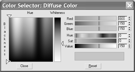
Select one of the material slots. Let’s change the color of the material. In the Blinn Basic Parameters rollout, click on the gray color swatch next to the Diffuse parameter. This opens the Color Selector dialog box, as shown in Figure 7-3.
Use the sliders on the right to set the red, green, and blue values for the color, or control the color using the Hue, Sat (Saturation), and Value levels.
You can also very easily select the desired color from the gradient on the left by dragging your mouse pointer over the colors until you find one you prefer. It’s best to pick the general color you need from the swatch on the left and then tweak the exact color by using either the RGB or the HSV controls on the right. The Hue of a color represents the actual color itself. Saturation defines how saturated that color is. Value sets how bright the color will be.
Once you have a color you like, click OK. If you want to restart the color, press Reset to zero out any changes. You’ll notice that the ambient color has changed as well as the diffuse color. You will see why in the next section, on the Material Editor itself.
In addition, you can add textures to almost any of the parameters for a material. Notice the blank square icon next to the Diffuse color swatch. Click that icon, and you will get the Material/Map Browser, which will be discussed later in the chapter.
The Material Editor is the central place in 3ds Max where you do all of your material creation and editing. You create materials to assign to any single object or group of objects in the scene. You can also have different materials assigned to different parts of the same object. In a full scene, it’s customary to have many different materials.
In 3ds Max 2011, there are two interfaces to the Material Editor: the Slate Material Editor (or Slate) and the Compact Material Editor.
Slate Material Editor
The Slate is a dialog box in which materials and maps appear as graphical nodes that you can connect or “wire” together to create material trees. In general, the Slate is more versatile than the Compact Material Editor when designing materials, while the Compact interface is more convenient when applying materials that have already been designed. If you are designing new materials, for example, the Slate is especially powerful since it gives a graphical view into how maps and materials are connected. The Slate (Figure 7-4) also includes search tools to manage scenes that have a large number of materials.
Get to know how the Slate works first, then get to know the types of materials and shaders in 3ds Max. Open the Slate by choosing Rendering ⇒ Material Editor ⇒ Slate Material Editor or by pressing the hot key M.
The main elements of the Slate are described in the following sections:
Material/Map Browser
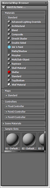
Running vertically on the left of the Slate is the Material/Map Browser shown in Figure 7-5. The Material/Map Browser interface is a list of materials, maps, and controllers, organized by libraries and groups that you can use in your scene. As shown in Figure 7-5, each library and group has a rollout to expand and contract the list, organizing the various material elements you can create.
Figure 7-4: The Slate Material Editor
Material/Map Browser Display
The Material/Map Browser is not only a part of the Slate, but can also be its own dialog box. Simply click and drag the top of the Material/Map Browser to undock it from the Slate. You can double-click its title bar to dock it. Additionally, the Material/Map Browser displays only materials and maps compatible with the currently active renderer. When using the Default Scanline Renderer for example, only Standard materials and maps are available. When using the mental ray renderer, more material and map options are available.
Materials
Materials are assigned to objects in the scene and give the geometry renderable qualities, such as color, transparency, and shininess. How you create your materials defines what the scene’s objects will look like when lighted and rendered. Different materials have different uses. You can even combine the effects of different materials using a material node called Blend. For example, a Blend material will mix together the results from two different materials for a compound effect, giving you incredible power in creating the surface look of your objects.
Figure 7-5: The Material/Map Browser
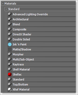
The Standard material types are shown in Figure 7-6.
Figure 7-6: Standard material types
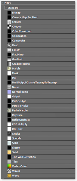
Maps
Maps allow you to apply bitmap image file textures or procedural textures to almost any parameter of a material. Maps create interesting looks by affecting color, transparency, bumpiness, and reflection.
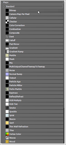
Bitmap images are images and pictures on your computer, such as a JPEG photo, while procedural textures are texture maps created and easily edited within 3ds Max, such as a checker pattern. Maps are shown in Figure 7-7.
Figure 7-7: Maps
Controllers
Controllers are nodes that control animation values on any given parameter for a material or map. For instance, if you wish to show an object slowly fade away, you can animate the value for the material’s transparency. These nodes make it possible for 3ds Max to have animated parameters and are only shown in the Slate.
Scene Materials
The Scene Materials rollout lists the materials (and sometimes maps) that are already being used in the scene (i.e., they have been assigned to an existing object in the scene). By default, it is always updated so it shows the state of the current scene. This is the best place to find and edit the materials in your scene.
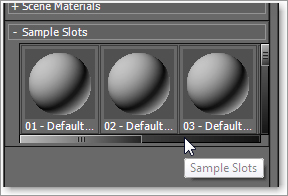
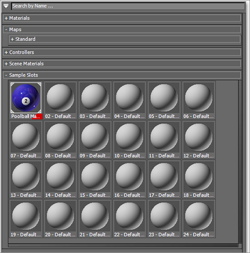
Sample Slots
The Sample Slots rollout (Figure 7-8) is a sampling of the materials with which you can work. The Slate’s Sample Slots section is a smaller version of the one seen in the Compact Material Editor, which you will see later in this chapter. This is a sort of “scratch pad” area where you can work on materials that are not yet part of the scene.
Figure 7-8: Sample Slots rollout
Active View
The Active View (shown in Figure 7-9) is where you design materials and lay out material node trees for the materials you want assigned to your scene objects. You construct material trees by double-clicking on a material in the Material/Map Browser section, such as a Standard material. You can also drag a material or map from the Material/Map Browser directly into the Active View.
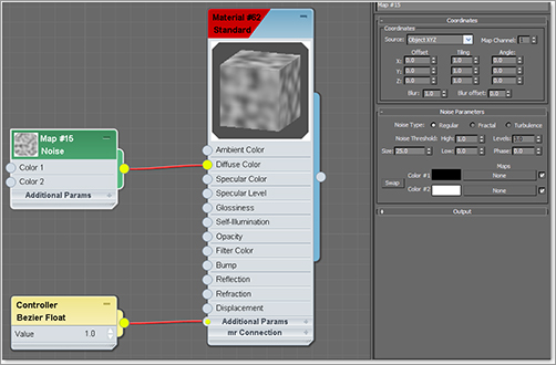
In Figure 7-9, we’ve created an oak material to assign to a CG surface in the scene. First we created a Standard material. Then we dragged a bitmap node (from the Maps Standard rollout) from the Material/Map Browser directly onto the little dot to the left of the Diffuse Color parameter on that Standard material. We chose the Oak Wood image file from 3ds Max’s installed library, giving the material its wood texture and color. This is called making a connection, or wiring; the bitmap (picture of the oak wood) is wired to the Diffuse Color parameter. Next we wired a Noise texture node to the Bump parameter to give the material some bumpiness.
Figure 7-9: The Active View shows a Standard material with maps wired to several parameters.
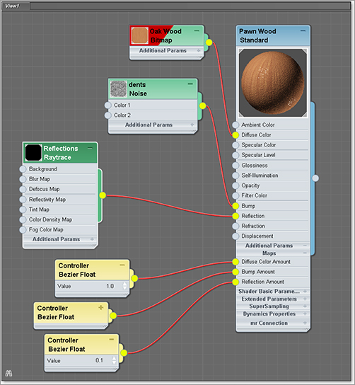
Finally we wired a Raytrace node to the Reflection parameter of the Standard material so 3ds Max would render reflections of the rest of the scene in the surface of this material’s object (for instance, a table top). As you can see in Figure 7-9, these nodes show clear connections so you can graphically see how the material works. The three nodes called Controller are created by 3ds Max by default and always appear as soon as you wire any maps to a material’s parameters. They are for creating animations of the settings for the maps and are otherwise ignorable.
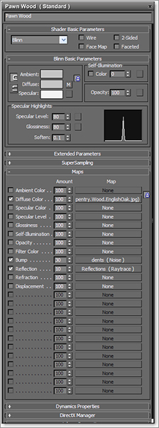
Figure 7-10: Parameter Editor
The node display for the Standard material in Figure 7-9 shows a listing of parameters under the title of the node, such as Ambient Color, Diffuse Color, and Specular Color. Each of these entries is called a Nodeslot or simply slot. When a map is connected to a parameter, you see a red curved line from the texture’s output slot to the material’s input slot, turning the slot’s dot yellow.
This is merely an introduction to the Slate; we will cover in much more depth how to create and edit materials using the Slate later in the chapter.
The keyboard and mouse controls for navigating the Active View are the same as those for navigating in the viewports. Furthermore, navigation tool icons are located at the bottom-right corner of the Slate. There is also a Navigator window in the Slate similar to the one used in Adobe Photoshop when you have a large number of nodes in the Active View.
You can also have multiple views to organize sets of material trees. Simply right-click by the tab named View1 in the Active View and choose Create New View from the context menu. We will use multiple views later in the chapter.
Parameter Editor
This is the area where you change the parameter values for your materials and maps. This will be explained further below and is shown in Figure 7-10.
Toolbar
You will find access to a variety of commands in the Slate’s toolbar. Many of these commands can be accessed through the Slate menu bar as well. The toolbar also has a drop-down list on the far right that lets you choose among multiple views.
Select Tool (![]() ) Speaks for itself—it selects! The hot key is S.
) Speaks for itself—it selects! The hot key is S.
Pick Material from Object (![]() ) An eyedropper cursor is displayed in the viewports when the tool is active. Click on an object in a viewport, and its corresponding material is displayed in the current Active View for editing.
) An eyedropper cursor is displayed in the viewports when the tool is active. Click on an object in a viewport, and its corresponding material is displayed in the current Active View for editing.
Assign Material to Selection (![]() ) Use this button to assign the selected material in the Slate to the object(s) you already have selected in a viewport. Also, you can drag a material’s output dot from the Slate to an object directly in a viewport.
) Use this button to assign the selected material in the Slate to the object(s) you already have selected in a viewport. Also, you can drag a material’s output dot from the Slate to an object directly in a viewport.
Delete Selected (![]() ) This deletes any material or map nodes that you have selected in the Active View and removes them from the Active View. It does not delete them from the scene. You may also press the Delete key.
) This deletes any material or map nodes that you have selected in the Active View and removes them from the Active View. It does not delete them from the scene. You may also press the Delete key.
Move Children (![]() ) When Move Children is on, moving a parent node moves the child nodes along with the parent. This means any materials with wired connections to maps, for example, will move the entire tree when you click and drag the material node, not just the material. This is similar to the animation exercise of the mobile and its hierarchy from Chapter 8, “Introduction to Animation.” The default is off and the hot key is Alt+C.
) When Move Children is on, moving a parent node moves the child nodes along with the parent. This means any materials with wired connections to maps, for example, will move the entire tree when you click and drag the material node, not just the material. This is similar to the animation exercise of the mobile and its hierarchy from Chapter 8, “Introduction to Animation.” The default is off and the hot key is Alt+C.
Hide Unused Nodeslots (![]() ) When a node is selected, this icon toggles how many of the slots for that node are displayed. When off, all of the node’s parameter slots are visible. When on, any slot that is not wired to another node is hidden. Default is off and the hot key is H.
) When a node is selected, this icon toggles how many of the slots for that node are displayed. When off, all of the node’s parameter slots are visible. When on, any slot that is not wired to another node is hidden. Default is off and the hot key is H.
Show Standard Map in Viewport (![]() ) This will display a material’s texture map in the viewport that is set to display Smooth + Highlights, so you can see the map on your model as you work in the scene. This is extremely helpful in positioning and sizing textures, as well as viewing your objects’ textures without rendering them. Lighting, however, is not taken into account here, so rendering is still the best way to see exactly how your scene will come out.
) This will display a material’s texture map in the viewport that is set to display Smooth + Highlights, so you can see the map on your model as you work in the scene. This is extremely helpful in positioning and sizing textures, as well as viewing your objects’ textures without rendering them. Lighting, however, is not taken into account here, so rendering is still the best way to see exactly how your scene will come out.
Show Background in Preview (![]() ) When you are working with transparent materials, turning on Show Background in Preview will place a multicolored checkered background in the Preview window for that material.
) When you are working with transparent materials, turning on Show Background in Preview will place a multicolored checkered background in the Preview window for that material.
Layout All flyout (![]() ) This flyout icon lets you choose between a vertical or a horizontal layout for the nodes in your view. Hold down the mouse button to access the other icon under the flyout.
) This flyout icon lets you choose between a vertical or a horizontal layout for the nodes in your view. Hold down the mouse button to access the other icon under the flyout.
Layout Children (![]() ) When you have a complicated material tree, this button automatically lays out all the child nodes for the material in an easy-to-read fashion. The hot key is C.
) When you have a complicated material tree, this button automatically lays out all the child nodes for the material in an easy-to-read fashion. The hot key is C.
Material/Map Browser (![]() ) Toggles display of the Material/Map Browser. The default is on and the hot key is O.
) Toggles display of the Material/Map Browser. The default is on and the hot key is O.
Parameter Editor (![]() ) Toggles display of the Parameter Editor. The default is on and the hot key is P.
) Toggles display of the Parameter Editor. The default is on and the hot key is P.
Select by Material (![]() ) When you have a selected material in the Slate and you click this button, all the objects assigned to that material are selected for you in the viewports.
) When you have a selected material in the Slate and you click this button, all the objects assigned to that material are selected for you in the viewports.
Compact Material Editor
The Compact Material Editor is the interface you are ready familiar with if you have used the program before this current version. This is a smaller dialog box than the Slate that gives you quick previews of various materials, without the node display (Figure 7-11.).
You can open the Compact Material Editor by opening the Slate and then in the Slate’s menu bar, selecting Modes ⇒ Compact Material Editor. You can switch back to the Slate through the same Modes menu.
Figure 7-11: The Compact Material Editor
Figure 7-12: Sample slot number options
Sample Slot The sample slot provides you with a quick preview of your material. Each material is displayed on a sphere in one of the tiles (or slots) in the Material Editor dialog. Right-clicking on any of the materials will give you a few more options, including the ability to change how many sample tiles you can see in the Material Editor (as shown in Figure 7-12). The fewer the samples, the quicker the Material Editor will load.
Get Material This button brings up the Material/Map Browser. Here you can browse from the scene or from a Material Library. The Material Library stores a collection of saved materials that you can bring into the current scene. You can use 3ds Max’s default materials or create your own and store them in your own custom library.
Assign Material to Selection You can use this button to assign the material to the selected object(s) in the scene. You can also apply materials by clicking and dragging the sample sphere from the Material Editor directly onto the object in the viewport; however, this can be less accurate, especially if you have a lot of objects.
Reset Map/Mtl to Default Settings This function resets the values for the map or material in the active sample slot.
Put to Library You can save your material to a library using this function. Building up a library of useful materials can save time, especially when you’re trying to re-create complex materials. Once you’ve gotten a material just right, there’s no reason you shouldn’t save it to your library by using this button.
Material ID Channel Here you can assign an effect ID to the material. Effects are used in the video post or the Combustion plug-in for things such as glow, highlights, and so on. Some of these effects will be covered in Chapter 11, “3ds Max Rendering.”
Show Standard Map in Viewport This will display your texture map in the viewport. This means that you won’t have to render every time you want to see how your material appears on a 3D object. However, displaying your map in a viewport has limitations. The limitations are basically those of your graphics card and your chosen method of displaying 3D in the viewport (Open GL, Direct3D, or Software). The difference between viewing the map in the viewport and in its final rendered state may be quite different. However, seeing a map in the viewport is useful on many levels.
Go to Parent Just as you created objects that related to each other, materials in 3ds Max may have several components to them (such as texture maps) that work in a hierarchy, where information from one node is fed upstream into the parameter for the material. When you are working with sub-maps, this option will take you back to the base material. This makes it easier to navigate in the Material Editor when you are editing your materials.
Go Forward to Sibling This option will take you into the next map channel; a lateral move from map to map.
Preview type Sometimes the default sphere won’t give you an adequate preview of the material. You can change the preview to a cube, a cylinder, or an object.
Pick Material from Object When you need to edit a material on an object, you can use this button to select the material from an object in the scene. The material is placed in the active sample slot.
Material name This is the name you give a material. This should be a descriptive name for the material that will instantly tell you what the material is for. 3ds Max will automatically give new materials a default name, such as the name 03, but it’s recommended that you change the material name from the default. You should do this before you apply it to an object, when you are adjusting the parameters (color, etc.) to suit your needs.
Material type Different materials have different uses. When called on to create a more complex material, for example, you can change the material type to Blend. A Blend material will mix the results from two different materials together for a compound effect. The default material type is Standard. Material types are explained later in this chapter.
Shader type Shader types describe how the surface responds to light. How an object looks depends on how its surface reacts to light, so the shader type for a material is very important. Shaders provide different options for specific materials. The default shader is Blinn. Shader types are covered later in this chapter. Not all material types let you specify different shaders.
Miscellaneous settings These are fairly basic settings used to change the appearance of the material. Here are two important settings.
Wire When you turn Wire on, the object attached to this material will render as a Wireframe object, as shown in Figure 7-13. This simple setting is very powerful; it’s used when you need to render line art or wireframe views.
Figure 7-13: The render as a Wireframe object (Wire on)

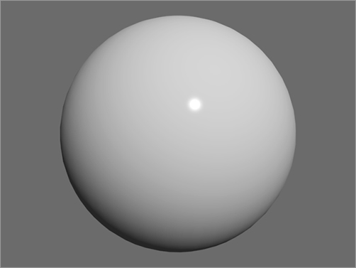
2-Sided This setting enables you to render both sides of a single surface. By default, only one side of a surface will render, and that is typically all you need. Sometimes, however, when you penetrate through a surface, you will have to see the other side. In Figure 7-14, a hemisphere is rendered without 2-Sided turned on. In Figure 7-15, 2-Sided has been enabled. Notice the inside of the hemisphere.
Locks Here you can lock the Ambient parameter to the Diffuse parameter and lock the Diffuse to the Specular. Any changes made to one while the locks are enabled affect both.
Figure 7-14: The render without 2-Sided enabled
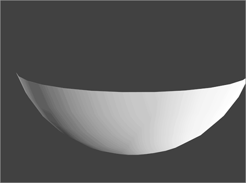
Figure 7-15: The render with 2-Sided enabled

Ambient, diffuse, and specular color Changing the ambient color will affect the way the material appears for ambient light. Changing the diffuse color affects the overall color of the material. Changing the specular color changes the color of the highlighted light. You change the color by clicking on the color swatch next to the parameter.
Diffuse and specular maps These buttons provide shortcuts to the maps for diffuse color and specular color. A map applied to diffuse color (for example: bitmap, which is an image file) will affect the base appearance of the material. A map applied to specular color will use the mapped image to define the location of the shine. Mapping is covered in the Pool Ball exercise later in this chapter, as well as in the rocket that we’ll texture.
Specular level map This setting determines how shiny the material appears. For something such as a metallic surface, the setting will be up around 180 to 220. You can also map a grayscale texture to determine which areas will appear shiny and which will appear dull.
Glossiness level map This setting determines the spread of the specular shine. A higher value means that it will look more plastic (high gloss across the surface of the model).
Self Illumination level map This slot creates the illusion of being lit from within. The more self illumination it is given, the less the material is affected by lighting, but the flatter it will appear.
Opacity level map A material’s opacity determines how transparent it appears. If it is set to 100 (the default), then the material is 100 percent opaque—that is, it’s solid. If it is set to 0, then it is completely invisible. You can apply a grayscale opacity map here that uses a bitmap (or other map) to define which portions of the material are transparent. Areas of white on the map will be opaque, whereas the black areas will render transparent; the intermediate values of gray will have different levels of transparency.
Figure 7-16: Applying maps to these parameters further defines the look of your material.
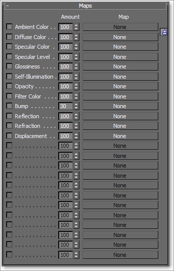
Maps rollout Maps allow you to apply bitmap or procedural textures, which help define the material beyond simple color and opacity settings. Common maps include bump maps (use grayscale values to simulate bumps and dents), displacement maps (use grayscale maps to mathematically calculate depth and height and redefine the mesh accordingly), reflections, glossiness, and so on, as shown in Figure 7-16.
Figure 7-17: Choose the material type from the Material/Map Browser.

Standard Material Types
Now that you’ve seen how the Slate and the Compact Material Editor work, let’s look at the different materials in 3ds Max. Different materials have different uses. The Standard material is fine for most uses. However, when you require a more complex material, you can change the material type to one that will fit your needs. To change a material type in the Slate, just choose from the list under the Materials rollout. By default, you will see a rollout for Standard. If you switch to a different renderer, for example mental ray, you will have other material type options. For example, using mental ray will give you access to a rollout for mental ray and MetaSL materials, as shown in Figure 7-17. The list is extensive, so we will touch on some of the best for an introduction here. We will also be showing examples using the Slate.
Standard
Standard material is the default type for the materials in the Material Editor. This material has values for ambient, diffuse, and specular components. With it, you can imitate just about any surface type you can imagine. The more advanced surface types (see the following discussions) combine elements of different shaders for more complex effects (Figure 7-18).
Figure 7-18: Standard material
Blend
Just as it sounds, this material type blends two materials together. Figure 7-19 shows the parameters for a Blend material type. Notice the controls for mixing two different materials. You assign the materials through the Material 1 and Material 2 parameters.
Composite
Similar to the Blend, a Composite material combines up to 10 materials, using additive colors, subtractive colors, or opacity mixing (Figure 7-20).
Figure 7-19: The Blend material type allows you to mix two different materials together.

Figure 7-20: The Composite material type allows you to blend up to 10 materials.

Double Sided
The Double Sided material type divides the material into two sub-materials, one for the outward face (Facing) and one for the inner face (Back). Figure 7-21 shows the parameters for the material.
In Figure 7-22, one material is assigned to the outer face of an object and another one is assigned to the back of the surface. Here, a bowl has a solid blue material mapped to the outside, and the inside face is a checker pattern map.
Figure 7-21: A Double Sided material allows you to assign different materials to either side of an object’s surface.

Figure 7-22: One material is assigned to the outer face and another material is assigned to the back.

Neither the facing nor the back material need to have 2-Sided enabled for the Double Sided material to render both sides of the surface.
Ink ’n Paint
Ink ’n Paint is a powerful Cartoon material that creates outlines and flat cartoon shading for 3D objects based on falloff parameters. Figure 7-23 shows the parameters for an Ink ’n Paint material.
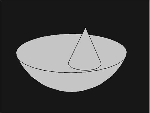
Figure 7-24 shows you a sample render with the Cartoon shading material applied to a bowl and a cone.
Figure 7-23: The Ink ’n Paint material’s parameters

Figure 7-24: A Cartoon-shaded render using the Ink ’n Paint material
Matte/Shadow
Use Matte/Shadow material when you want to isolate the shadow. The material will receive shadows, but it will remain transparent for everything else. It is useful for rendering objects onto a photo or video background because it creates a separate shadow that you can composite on top of the background. Rendering in separate passes, such as a separate shadow, is very useful because you can have total control of the image by compositing just the right amount of any particular pass. The Matte/Shadow material is unavailable when mental ray is active; instead, use the Matte/Shadow/Reflection mental ray material.
Multi/Sub-Object
Use this material when you need to apply different materials to polygons of a 3D object. Material IDs are assigned either manually or automatically, depending on how you create the material. (This is covered later in the chapter.) Material IDs determine which sub-material is applied to which polygon. This lets you assign different surface treatments to a single object. This keeps modeling simpler because you do not have to make separate objects for everything that needs a different material.
Figure 7-25: The Raytrace material node gives you true reflections and refractions.

Raytrace
The Raytrace material is a powerful material that expands the available parameters to give you more control over photo-real renderings. The material uses more system resources than the Standard material at render time, but it can produce more accurate renders—especially when true reflections and refractions are concerned (Figure 7-25).
Shellac
The Shellac material superimposes one material on another using additive composition. This allows you to create a material that is highly glossy, such as a finely varnished wood surface (Figure 7-26).
Top/Bottom
Top/Bottom divides the material into a top material and bottom material with an adjustable position (Figure 7-27). This material is useful for creating an object that has two different materials on either side, such as a cookie with chocolate on the top.
Figure 7-26: The Shellac material allows you to superimpose a shiny layer on top of another material.
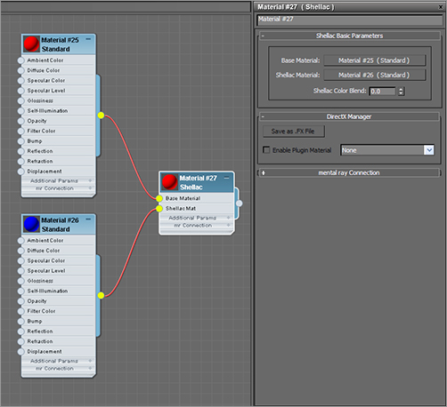
Figure 7-27: The Top/Bottom material type

mental ray Material Types
3ds Max comes with several materials that are created for use only with the powerful mental ray renderer. These materials are visible in the Material/Map Browser only when mental ray is the active renderer. In Chapter 11, we will further cover one of the mental ray materials, the Arch & Design material. Brief descriptions of a few mental ray materials are provided here.
Arch & Design
The mental ray Arch (architectural) & Design material is a material with a refined and high quality feel. Made for architectural renderings, this versatile material provides great glossy surfaces, such as polished floors, ceramics, enamel, and metals This material has special features, including advanced options for reflectivity and refractive transparency (Figure 7-28).
Figure 7-28: Arch & Design material node and parameters

Car Paint
This material simulates the look of a car’s surface when it is lighted properly. The material itself has a tremendous number of options and parameters, and is a an advanced material. In addition to the material, there are several lighting considerations to be made when rendering an object with the Car Paint material.
Subsurface Scattering Fast Material
The Subsurface Scattering (SSS) materials, including the Fast Material, simulates surfaces that absorb and diffuse light, such as wax, skin, or a sponge. These objects take in a certain amount of light and scatter the light through the surface for a definitive look. For example, a leaf that is backlit would use a Subsurface Scattering material. 3ds Max’s Subsurface Scattering Fast Material does a good and quick job of rendering such surfaces compared with the other SSS materials. The SSS materials are advanced materials that require quite a bit of rendering and lighting experience.
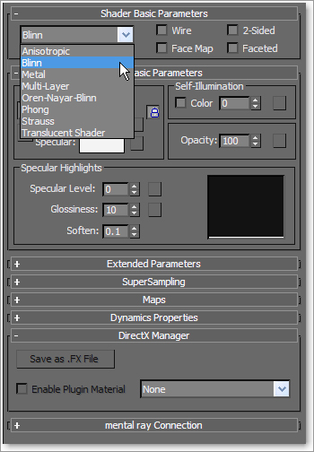
Figure 7-29: Shader types define the surface of the material.
Shader Types
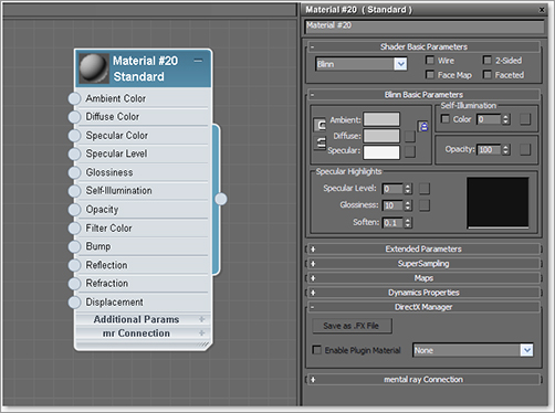
The way light reflects from a surface defines that surface to your eye. In 3ds Max, you can control what kind of surface you work with by changing the shader type for a material. In either the Compact Material Editor or the Slate Material Editor, you will find Shader Types as a pull-down menu in a material’s Shader Basic Parameters rollout, as shown in Figure 7-29. This option will let you mimic different types of surfaces, such as dull wood or shiny paint or metal. The following descriptions outline the differences in how the shader types react to light.
Figure 7-30: The Anisotropic shader
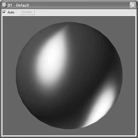
Anisotropic
Most of the surface types that you will see in this section typically create rounded specular highlights that spread evenly across a surface. By contrast, anisotropic surfaces have properties that differ according to direction. This creates a specular highlight that is uneven across the surface, changing according to the direction you specify on the surface. The Anisotropic shader (Figure 7-30) is good for surfaces that are deformed, such as foil wrappers or hair.
Figure 7-31: The Material Editor for the Anisotropic shader
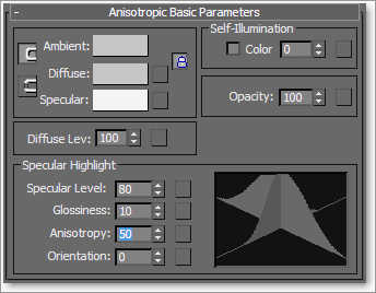
Figure 7-31 shows the Material Editor for an Anisotropic material. Notice the extra controls for the specular highlights. These allow you to control how the specular highlight will fall across the surface.
Blinn
This is the default shader in 3ds Max because it is a general-purpose, flexible shader. The Blinn shader (Figure 7-32) creates a smooth surface with some shininess. If you set the specular color to black, however, this shader will not display a specular highlight and will lose its shininess, making it perfect for regular dull surfaces, such as paper or an indoor wall. Figure 7-33 shows the Blinn shader controls in the Material Editor.
Figure 7-32: The Blinn shader
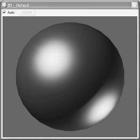
Figure 7-33: The Material Editor for the Blinn shader

Because this is the most-often used shader, let’s look at its Material Editor controls. The ambient color, and specular colors all work as you read previously in this chapter. You can set the color you want by clicking the color swatch, or you can map a texture map to any of these parameters by clicking the Map button and choosing the desired map from the Material/Map Browser.
Specular Highlight Controls
The parameters in the Specular Highlights section of the Blinn Basic Parameters rollout are interesting in this shader. The specular color, which defaults to white, controls the color of the highlight. Decreasing the brightness of that specular color, whatever the color may be, will decrease the brightness of the specular highlight on the object, making it seem less shiny. Changing the specular color to black will negate any surface shine.
The surface shine is also regulated by the Specular Level parameter. The higher the value, the hotter the specular highlight will render on the object. Figure 7-34 shows a sphere with a Blinn with a Specular Level of 0 on the left, 35 in the middle, and 100 on the right.
The Glossiness parameter controls the diameter of the specular highlight. With the same sphere with a Specular Level of 35, Figure 7-35 shows you a Glossiness of 0 on the left (which creates a broad specular highlight), a Glossiness of 35 in the middle (which creates a fairly tight, shiny specular highlight), and a Glossiness of 75 on the right (which creates a high gloss pinpoint specular highlight). The higher the value, the glossier the surface will appear.
Figure 7-34: The Specular Level parameter of the Blinn shader controls the amount of highlight on the surface.

Figure 7-35: The Glossiness parameter controls the diameter of the specular highlight.

Finally, the Soften parameter controls the softness of the specular highlight. Figure 7-36 shows a sphere with a Blinn material assigned with a Specular Level value of 55, a Glossiness value of 10, and a Soften value of 0 on the left and 1 (the max) on the right.
Figure 7-36: The Soften parameter helps rein in broad specular highlights by softening their edges.

Soften controls the specular breadth on specular highlights that are already broad—that is, they have lower Glossiness values. You may want to look at these parameters at work in a 3ds Max scene, as your monitor will display the specular highlights better than a printed page.
Figure 7-37: The Specular Highlights level graph shows the falloff of the specular highlights.

You’ve probably noticed the graph (shown in Figure 7-37) in the Material Editor when you work with the Specular Level, Glossiness, and Soften parameters. This graph shows you the falloff of the specular highlight you are editing for the material. The shorter the graph, the lower the level of specular highlight. The rounder the graph, the broader and softer the specular highlight.
For shiny objects, you will need to use a fairly sharp specular highlight. For extremely shiny objects, such as polished metals, a pinpoint specular highlight is best. Plastic objects will work best with a broad, diminished specular highlight. Matte objects, such as paper or cloth, work great without a specular highlight, or at least a very darkly colored one.
Self-Illumination
The Self-Illumination parameter creates the illusion of incandescence on an object, meaning the object seems to be self-lit. The object’s darker areas (where it is not receiving direct light) will essentially take on the color specified for the Self-Illumination parameter.
The higher this value, the flatter the object will appear, because Self-Illumination will essentially negate any shadowing or ambient falloff on the material. The specular highlights on the material will still show up on a material with Self-Illumination turned all the way up to 100. You can also change the color of the Self-Illumination by clicking the Color check box and choosing a color in the swatch that appears when Color is enabled. This allows you to have a different self-illumination color than the color of the material itself. Figure 7-38 shows a Self-Illumination value of 0 on the left and a Self-Illumination value of 1.0 on the right. Notice how the sphere flattens out as Self-Illumination helps keep the shadow areas as bright as the diffuse areas.
Figure 7-38: The Self-Illumination value sets the incandescence of a material.
A Self-Illumination value does not emit a light in the Default Scanline Renderer—that is, the object will not illuminate other objects in the scene. For such an effect, you will need to use more advanced rendering techniques with mental ray, for example.
Opacity
The Opacity setting sets the transparency of an object. The higher the Opacity value, the more solid it renders. The lower the Opacity value, the more see-through the object will render.
Metal
Figure 7-39: A sphere with a Metal shader
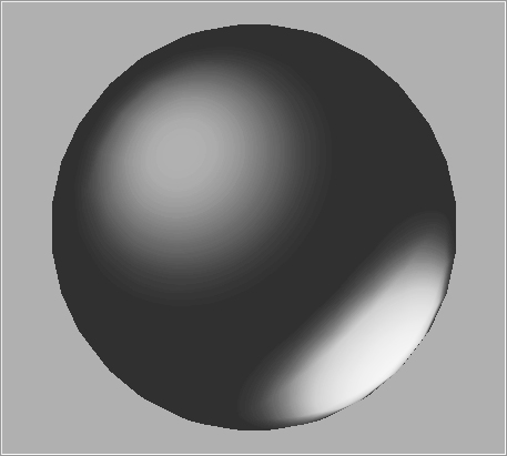
The Metal shader is not too different from the Blinn shader. Metal creates a lustrous metallic effect, with much the same controls as a Blinn shader, but without the controls for specular highlights. When you are first starting, it’s best to create most of your material looks with the Blinn shader until you’re at a point where Blinn simply cannot do what you need. Figure 7-39 displays a sphere with a Metal shader with a Specular Level of 120 and a Glossiness of 60.
The dark areas of the shader may throw you off at first, but keep in mind that a metallic surface is ideally black when it has no light, meaning there’s nothing to reflect. Metals are best seen when they reflect the environment. Given that, this shader requires a lot of reflection work to make the metal look just right.
Figure 7-40: A material with the Multi-Layer shader assigned to a sphere
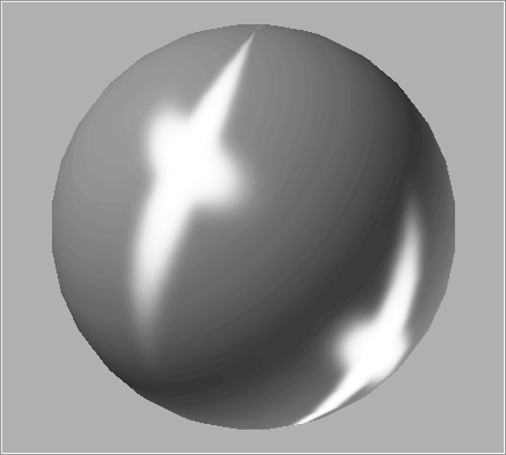
Figure 7-41: The Multi-Layer shader lets you create complex highlights.

Multi-Layer
With some surfaces, you need complex highlights. In some cases, while an Anisotropic shader might be useful, you may need further control in the complexity of your specular shape and falloff. A Multi-Layer shader will stack two Anisotropic highlights together to give you increased control over the highlights you can create.
Here you can see a material with the Multi-Layer shader assigned to a sphere (Figure 7-40).
The two layered specular highlights are created in such a way, as shown in Figure 7-41, to create an “X” formation for the highlights.
Oren-Nayar-Blinn
The Oren-Nayar-Blinn shader (Figure 7-42) generally creates good matte surfaces such as cloth or clay. The shader has specular highlight controls very similar to those of the Blinn shader.
Phong
The Phong shader (Figure 7-43) is a legacy shader that was created before the introduction of the Blinn shading model. The Phong shader looks very similar to the Blinn shader, and it has the same controls. Phong creates smooth surfaces with some amount of shininess, just as Blinn does. However, Phong does not handle highlights as well as Blinn. This is especially true for glancing highlights, where the edge of a surface catches the light. Phong is good for creating plastic objects, as well as many other surfaces.
Figure 7-42: The Oren-Nayar-Blinn shader

Figure 7-43: The Phong shader
Strauss
The Strauss shader (Figure 7-44) can create metallic and nonmetallic surfaces. Its main controls are Color, Glossiness, Metalness, and Opacity. The specular highlights, for the most part, are governed by the Glossiness setting of the material. The higher the Metalness value, the darker the unlit portions of the surface become, again relying on reflections for the metallic look.
Translucent Shader
Translucence is the degree to which light is scattered as it passes through the material—for example, when a flashlight shines behind a sheet of parchment. The Translucent shader (Figure 7-45) is very similar to the Blinn; however, this shader adds a touch of translucency to the material.
You can also simulate frosted and etched glass by using translucency. Figure 7-46 shows the Translucent Basic Parameters rollout for a Translucent shading material.
Figure 7-44: The Strauss shader

Figure 7-45: The Translucent shader

Figure 7-46: The Translucent shader allows light to scatter through the object.

Let’s put some of that hard-earned knowledge to work and map an object. You will be creating and texturing a pool ball. Although this may not seem the most exotic thing to texture, you can learn a lot about surfaces, shading, and mapping techniques by texturing it. You’ll be able to flex your mapping muscles even more in exercises later in the chapter.
Starting the Pool Ball
If you have skipped to this section from the beginning of the chapter, have a run through and get a good taste of texturing in 3ds Max. Feel free to look at the earlier parts of the chapter for some of the hows and whys of what you will accomplish in this exercise. Otherwise, roll up your sleeves and follow along with these steps to texture a pool ball.
You can begin with your own project, or you can copy the Pool Ball project you have downloaded from the web page at www.sybex.com/go/intro3dsmax2011. It contains texture image files you’ll need for this exercise.
1. In a new scene, create a sphere. The size doesn’t matter here. How’s that for fast modeling?
2. Open the Material Editor by pressing the hot key M or clicking the Slate Material Editor icon (![]() ) in the Main toolbar. If the icon isn’t visible, click and hold down on the Compact Material Editor icon to bring up a flyout, then choose the Slate Material Editor icon.
) in the Main toolbar. If the icon isn’t visible, click and hold down on the Compact Material Editor icon to bring up a flyout, then choose the Slate Material Editor icon.
3. In the Slate Material Editor, go to the Material/Map Browser, and from the list double-click on the Standard material type. This will add a Standard material node to the View area (Figure 7-47). Then double-click on the material node’s title bar to activate the material parameters on the right of the Slate.
Figure 7-47: Standard material in the Material/Map Browser

4. The most logical thing to start with is the color. The base color of an object is defined by the Diffuse parameter—although Ambient is also locked to Diffuse, which is fine.
5. Click on the color swatch to the right of the Diffuse parameter to open the Color Selector, as shown in Figure 7-48. Pick any color at this point. Once you have chosen your color, click the Close button, and you will see that the sphere icon at the top of the material node has changed to that color.
Figure 7-48: The Diffuse parameter color swatch

Choosing a Surface Type
The next step is to decide what the surface of your object will be. Will it be shiny or matte? You will need a shiny surface, because real pool balls are glossy. We will have to adjust the specular highlights using the Blinn’s controls.
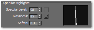
1. Go to Specular Highlights under Blinn Basic Parameters. Set the Specular Level to 98 and the Glossiness to 85. Keep Soften at the default. The specular graph in Figure 7-49 is quite sharp.
Figure 7-49: Specular Highlights settings for the pool ball
2. That is it for the basic material. Now apply the material to the object by dragging from the node’s output socket (the dot on the right of the material node, as shown in Figure 7-50) onto the object in the viewport. The sphere will change to the color you chose for the Diffuse parameter, and in the sample slots the corners will become outlined with white triangles.
Figure 7-50: Apply materials by dragging from the material node’s output socket to the object.
As a matter of fact, gray corner triangles on a sample slot in the Material Editors mean that the material is applied to an unselected object in the scene. When the corner triangles are solid white, the material is “hot” and its assigned object is currently selected, as shown in Figure 7-51. So you can see the nodes sample slot better, double-click the small slot next to the title bar to enlarge it.
Figure 7-51: Material node
The material in the editor is now the material assigned to the object. If you were to change any of the parameters of the material, it would be instantly updated on the object. Once you assign a material, there’s usually no need to return to the object’s default color, although you may find yourself replacing the material with another material frequently.
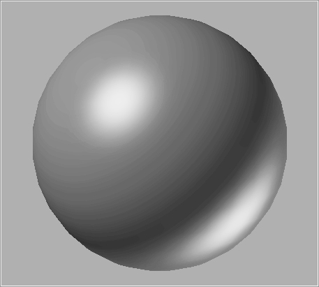
Figure 7-52 shows you what the pool ball should look like, most noticeably its specular highlight. However, viewing in the viewport isn’t the same as a rendered image. The viewport gives the lowest level of quality, and it should not be used to make final decisions on the look of your material. Instead, it should be used as a point of reference.
Figure 7-53 shows this pool ball rendered. Rendering (covered in detail in Chapter 11) combines the materials, lights, shadows, and environments within a scene to create the final look. Notice how much more detailed the specular highlight is in the render. To check your render, click the Render icon (![]() ) in the Main toolbar.
) in the Main toolbar.
Figure 7-52: The pool ball in a viewport
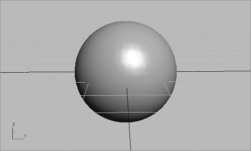
Figure 7-53: The pool ball rendered
Placing a Map on the Pool Ball
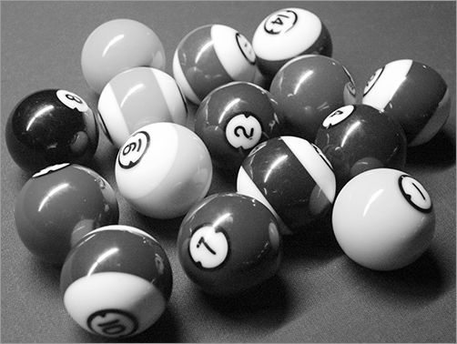
This simple material is only part of the story. Just creating a sphere and making it shiny and giving it color doesn’t make a realistic ball. Pool balls have a graphic stripe or number in a circle. You still need to add the markings of a real pool ball, not just a solid color. Figure 7-54 shows some real pool balls. You can’t create the needed detail using the basic parameters of the Standard material. What you need is a bitmap.
Figure 7-54: Pool balls
This procedure has to do with texture placement. As you gain more experience, you’ll learn how to prepare your texture images for your models. A bitmap replaces the diffuse color with an image. The image you use can be hand drawn and scanned, created in a program such as Adobe Photoshop, or taken with your digital camera. The image we are going to use (Figure 7-55) was created in Photoshop. A white circle with the number 2 is in the middle and one that is cut in half is on either side.
Figure 7-55: The proposed bitmap texture for the ball
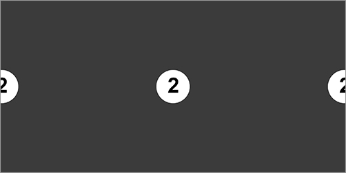
Figure 7-56: Choose Bitmap from the Material/Map Browser.
The theory behind this image is quite simple. Pool balls have the number on opposite sides of the ball. In your texture map, you’ll need to make two number 2s on the blue backdrop. The two halves of the white circle and the number 2 will simply tile together when the texture image wraps around the sphere, much like how a wrapper wraps around a piece of candy. This way you have two number 2s on the ball, easy as pie. To apply this bitmap as a texture, follow along here:
1. Go to the Slate and from the Material/Map Browser, click on the Maps ⇒ Standard rollout and either double-click or click and drag from Bitmap to the view area (see Figure 7-56). The Select Bitmap Image File dialog box immediately comes up.
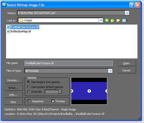
2. Navigate to the PoolBallColorTexture.tif file in the SceneAssetsImages folder of the Pool Ball project downloaded from the web page and copied to your hard drive. See Figure 7-57.
Figure 7-57: Choose PoolBallColorTexture.tif in the Select Bitmap Image File dialog box.
3. Now in the view area you should see a Bitmap node next to the Material node, as shown in Figure 7-58. These nodes still need to be wired together. Drag from the output socket of the Bitmap node to the input socket of the Diffuse Color slot (see Figure 7-59). When you make the connection, another node will be wired along with the bitmap node called a Controller node. A Controller node allows you to adjust or animate a map’s values. See Figure 7-60.
Figure 7-58: Bitmap node added to the view area
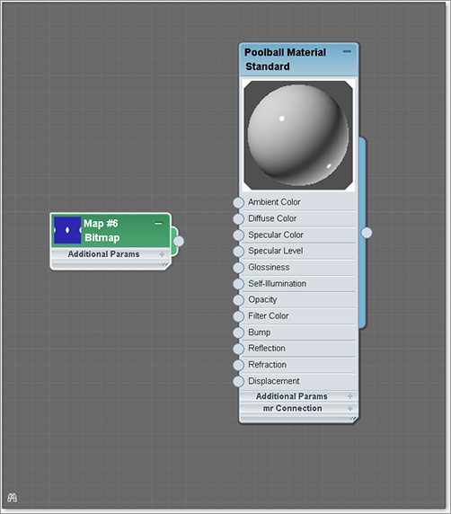
Figure 7-59: Linking the Bitmap node to the Standard material node, Diffuse Color

Figure 7-60: The Controller node is added.

Figure 7-61: The Slate shows the parameters for your bitmap image.
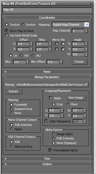
4. Double-click on the Bitmap node to bring up its parameters. There are several rollouts that we will ignore for now. The most important rollouts in the Bitmap section are Bitmap Parameters and Coordinates. The Bitmap Parameters rollout deals with the actual bitmap image; the Coordinates rollout controls how the bitmap image moves relative to the surface of the object. Leave all the settings at their defaults. See Figure 7-61.
If you ever need to change a bitmap image in a texture already applied, simply go to the bitmap’s parameters and under the Bitmap Parameters rollout, click on the bar with the filename to the right of the Bitmap parameter. The file browser will reopen. Choose another image file, and it will replace the current bitmap file.
5. You will be able to see the bitmap in the sample slot, but not in the viewport. To fix this, click the Show Standard Map in Viewport button (![]() ) on the Slate’s toolbar at the top of the Slate’s interface below the menus.
) on the Slate’s toolbar at the top of the Slate’s interface below the menus.
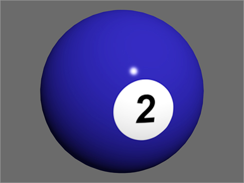
6. Now render the ball to check the map’s appearance. With your Perspective viewport active, click the Render icon (the teapot). Figure 7-62 shows the pool ball with the mapping.
Mapping Coordinates
When you put a 2D image onto a 3D object, think of it as being “projected” onto the surface, as if you had a white object and a slide projector were projecting a picture onto the white surface. Mapping coordinates describe how the image is projected or wrapped around the surface. Coordinates are spelled out in terms of U, V, and W. U is the horizontal dimension, V is the vertical dimension, and W is the optional depth. All primitives have mapping coordinates, including our sphere. That doesn’t necessarily mean the image will wrap itself correctly, although it works fine for our Pool Ball exercise (imagine that!). Merely having the mapping coordinates only means the map will show up. To edit the mapping coordinates, you need to use the Coordinates rollout. You will learn more about mapping coordinates as well as UV unwrapping work later in this chapter.
Figure 7-62: The ball with the mapped image
Adding a Finishing Touch—Reflection Mapping
With the image applied, the pool ball looks pretty good at this point (Figure 7-62)—but it can be better. The small nuances are what really make a render look good. One thing this pool ball is missing is a reflection of its environment. Now, short of creating and texturing a pool table and several other pool balls, we need to make a cheat.
There are two ways to create reflections: the “faking it” method (using mapping) and the raytrace method. Both methods require us to go to the Maps rollout in the Material Editor. We are going to use the cheat and add a bitmap into the Reflection map slot. We are going to use the “faking it” method.
Raytrace is a rendering methodology that traces rays between all the lights in the scene with all the objects and the camera. It can provide true reflections of objects in the scene. Chapter 11 covers raytracing in more depth.
To fake the reflection, you’ll need an image that looks like the “room” around the ball. We are going to use a photograph taken for this occasion and saved as the image file ReflectionMap.tif in the SceneAssetsImages folder of the Pool Ball project from the companion web page (Figure 7-63).
Figure 7-63: The reflection map used to “cheat” the reflections on the pool ball
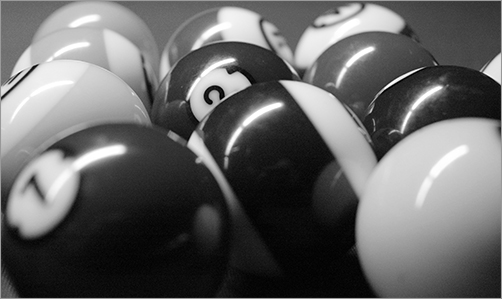
This image has all the elements that you might see around a pool ball—specifically, more pool balls! To add this image as a reflection for the ball, follow these steps:
Figure 7-64: The reflections are a bit heavy. If you could reduce the amount of reflection, they’d be better.

1. Go to the Slate and in the Material/Map Browser, drag a bitmap into the view area. Navigate to ReflectionMap.tif in the SceneAssetsImages folder of the Pool Ball project you downloaded to your hard drive, then click the Open button.
2. In the view area drag from the output socket of the Bitmap node to the input socket of the Reflection slot.
3. Do a quick test render with the Render icon (the teapot icon in the Main toolbar). The reflections are pretty strong (Figure 7-64).
4. You need to adjust how much reflection is on the ball. In the view area, go to the Controller Bezier Float node connected to the Reflection Amount parameter, expand the node by clicking on the plus sign next to the title. Change the Value to 0.2 as shown in Figure 7-65. Test-render the pool ball again. You should notice a much nicer level of reflection (Figure 7-66). Voilà! Save the file.
Figure 7-65: Change Value in the Controller Bezier Float to 0.2.
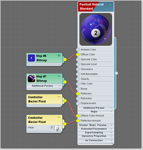
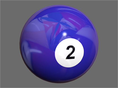
Figure 7-66: The reflections look much better and add realism to the pool ball.
If you have lost the view of your pool ball somehow, or if you simply want to center it in the Perspective viewport (or any other viewport), press the Z shortcut to focus the viewport on all the objects in the scene. In this case, it will center the pool ball.
Background Color
Figure 7-67: The Environment and Effects dialog lets you change the background color.

You may notice that the background in the renders in Figures 7-64 and 7-66 is gray, whereas your renders’ backgrounds are (probably) black. There are many reasons why you would want to control the background color, which you can do with a simple setting change. You may want a specific color to offset your scene (for example, blue to represent the sky) or you may want a picture in your background.
To change the background of your renders, go to the Main Menu bar and choose Rendering ⇒ Environment. The Background parameter is at the top of the dialog box (Figure 7-67). Click on the color swatch and choose your color. That’s it!
To add an image to the background, click on the bar marked None to add a bitmap, just as you did with the bitmaps on the pool ball. Once you do, the image will render in the background with your scene. To change the image, click that bar (which at that point should list the path and filename of the current image) to go to the Material/Map Browser, where you can select a new bitmap and image.
Mapping, Just a Little Bit More
Now that you know how to add maps to a material, removing them is very simple. In the Compact Material Editor for the parent material’s parameters (not the map’s parameters), right-click on the map name and select Clear from the context menu, as shown in Figure 7-68.
If you don’t want to clear the map entirely, but just need to turn it off for a little while, you can just uncheck the box to the left of the parameter name, as shown in Figure 7-69. Check it again to use that map again.
In the Slate, selecting a map’s node and pressing Delete on your keyboard will disconnect the map from the material, but will also delete the map node itself along with its Controller node. If you wish to temporarily disconnect a node, simply click on the connecting wire between the nodes to select it, and then press Delete. This will delete the connection, but keep the nodes intact though disconnected. You can simply rewire the connection between the nodes as needed.
Figure 7-68: Removing a map from a parameter
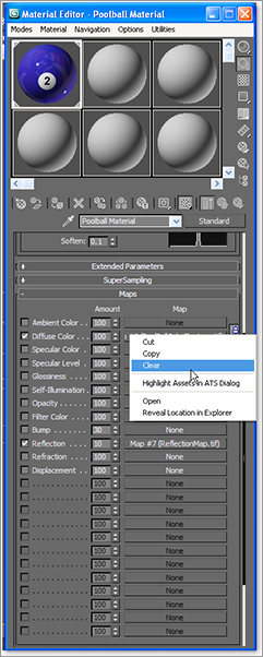
Figure 7-69: Unchecking the box next to a mapped parameter will temporarily remove the map from the parameter.

Seeing More Sample Slots
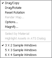
In the Compact Material Editor, if you have a scene with several materials, and you need to see more sample slots than the default in the Material Editor, simply right-click on any slot and select either 5 × 3 Sample Windows or 6 × 4 Sample Windows from the context menu. See Figure 7-70. This will help you navigate a heavy scene that has tons of materials that you need to modify. In the following figures, you can see the sample slots multiply!
Figure 7-70: To show more sample slots in the Compact Material Editor, use the right-click menu and choose either 3 × 2, 5 × 3, or 6 × 4 rows.
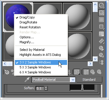
Figure 7-71: Magnify gives you a larger view of your material.

Figure 7-72: The Sample Slots rollout in the Slate Material Editor
As you’ve seen, the sample slots for any given material in the Material Editor constantly update to show you any changes you’ve made to that material. However, if you want a larger image than the relatively small sample slot, double-click on the slot or right-click on the slot and select Magnify from the context menu. A larger window (Figure 7-71) opens (which is resized by dragging the corners of the window) with a sample of that material. By default it will update automatically as you make changes to the material.
You’ve already noticed that there are at most only 24 sample slots in the Compact Material Editor when you expand to 6 × 4 Sample Windows as in Figure 7-70. This does not limit to 24 the number of materials you can use. You should consider both Material Editors as a scratchpad of sorts. You can create as many materials as you’d like in a 3ds Max scene; however, only 24 can be loaded in the Material Editors at the same time.
If you click the Get Material button in the Compact Material Editor, you can list all the materials that are used in the scene. When the Material/Map Browser is open, click to expand the Scene Material rollout for the Browse From parameter, and all of the materials assigned in the scene will be listed. When an object’s material is not shown in a sample slot, it does not mean it has been deleted. You can load it back into any sample slot for editing at any time.
For the Slate, in the Material/Map Browser you can see the Sample Slots rollout. All 24 slots are visible, as shown in Figure 7-72. This also applies to the Compact Material Editor.
Assigning Materials to Sub-Objects
You’ve seen several times how to assign a material to an object. You can, for instance, drag from the output socket of the material node in the Slate to the object in a viewport or, if you are using the Compact Material Editor, you can drag the sample slot with the material you created onto the object in your scene. You can also select an object in the viewport, and then select a Sample Slot material and click the Assign Material to Selection button (![]() ) in the both Compact and Slate Material Editors.
) in the both Compact and Slate Material Editors.
You may want to assign materials to sub-object polygons as well as whole objects. One approach is to use the Multi/Sub-Object material type briefly discussed earlier in the chapter.
There is a much easier way to assign materials to sub-objects, however. Just select the appropriate polygons on the surface (the object must be an Editable Poly or have an Edit Poly modifier applied), and assign the material as you regularly would (using the Assign Material to Selection button or dragging the material or the wire from the output of the material node to the selected polygons in the viewport). A sphere with several polygons assigned to different materials is shown in Figure 7-73.
Figure 7-73: Applying materials to a mesh’s sub-object polygons is easy.

Once you apply a material to a sub-object, a new Multi/Sub-Object material is created in the scene automatically. You can load the new Multi/Sub-Object material by using the eyedropper to click on the object in the viewport to load the material into a sample slot.
Exploring the Various Map Types
By now you’ve noticed that the Material/Map Browser has different maps you can access (as shown in Figure 7-74). The most popular map types are described here.
Figure 7-74: The Material/Map Browser has many different maps.

2D Maps
2D maps are two-dimensional images that are typically mapped onto the surface of geometric objects or used as environment maps to create a background for the scene. The simplest 2D maps are bitmaps; other kinds of 2D maps are generated procedurally.
Procedural maps are generated entirely within 3ds Max and rely on a set of parameters you set for their look. Images brought in the way the pool ball’s color and reflection maps were brought in are not procedural maps. They are bitmaps—that is, raster image files. For more on raster image files, see Chapter 1, “Basic Concepts.”
Click on the Standard Maps category in the Material/Map Browser to see the available 2D maps.
Bitmap
As you’ve already seen, a bitmap is an image file that you load into 3ds Max. It can be a photo, a scan, or any image that is readable by 3ds Max.
Checker
A procedural map, the checker map is a checkerboard pattern that is generated in 3ds Max. Its parameters in the Slate (shown in Figure 7-75) control the look of the checkerboard.
Figure 7-75: The checkerboard pattern
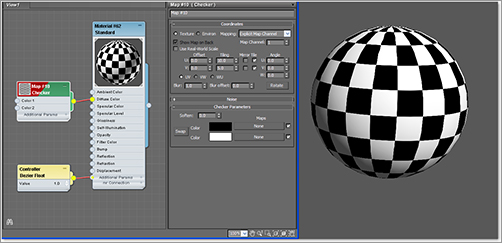
The Tiling values under the Coordinates rollout determine the number of checkers. The higher the number, the more checkers. The two color swatches, of course, control the two colors of the checkerboard; black and white are defaults. You can either click the color swatch to change the color, or you can click the Map bars (labeled None until you assign a map) next to each color. The Blur parameter allows you to blur the edges of the checkers, and the Soften parameter under the Checker Parameters rollout blurs the checkers together.
Gradient
A gradient is a procedural map (the parameters are shown in Figure 7-76) that grades from one color to a second color to a third color.
In the Coordinates rollout, the parameters are much the same as they are for the checker map. These coordinates are pretty much the same for all procedural maps, as they allow you to position the map as you need on the object by setting the options such as Tiling and Offset.
Figure 7-76: The gradient map

The colors for the gradient are set by Color #1, Color #2, and Color #3. You can also map these colors. The Color 2 Position parameter sets the relative location of the middle color to the upper and lower colors—i.e., 0.5 is the middle because the other colors are at 0 and 1.0.
Figure 7-77: Preview Object Type changes the shape of the object in the material preview window.

Notice the material preview that used to be a sphere is a cylinder. You can change the object type from the right-click menu. Right-click on the material node, go to Preview Object Type, and choose Cylinder (Figure 7-77).
Gradient Ramp
Similar to the Gradient map, but much more powerful, the Gradient Ramp is a procedural map that allows you to grade from and to any number of shades. Gradient Ramps are perfect for creating maps that fall off (for example, for opacity effects where the opacity fades away). See Figure 7-78.
Use the sliders along the ramp in the Gradient Ramp Parameters rollout to set the position of the gray value. Click in the ramp to create a new slider at that grayscale value. The black and white sliders at the very ends do not move. To delete a slider, right-click on it, and choose Delete from the context menu that appears. Notice the value and position readout above the ramp. As you can see in the view area, the more colors added to the ramp, the more controllers added to the Gradient Ramp node. It gets pretty messy! If you want only the children to the Gradient Ramp hidden, right-click on the node and from the menu choose Hide Child Tree (Figure 7-79).
Figure 7-78: The Gradient Ramp node
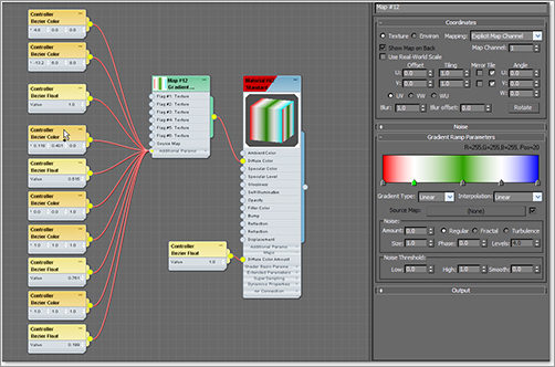
Figure 7-79: The right-click menu for the Gradient Ramp node
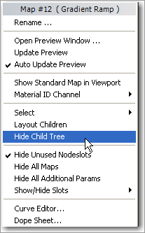
You don’t necessarily need the controller showing because you can edit the color through the material’s Parameters menu. When you finish designing the material, you may want to hide all the materials children, so right-click in the view area, choose Hide Children from the menu, and the material node’s children will be hidden.
3D Maps
Similar to 2D maps, which are generated in two dimensions, 3D maps are patterns generated procedurally in all three dimensions. For example, Marble has a grain that goes through the assigned geometry in X, Y, and Z. If you cut away part of an object with Marble assigned as its texture, the grain in the cutaway portion matches the grain on the object’s exterior.
When you create a 3D map, notice that the Coordinates rollout has Tiling and Offset parameters in three axes, whereas the 2D maps have only U and V.
Try using some of the 3D maps (such as Marble, Noise, and Wood) to see how they work on a simple object in your scene. They all have basically the same Coordinates rollout; however, each has its own Parameters rollout to control the color and other settings.
Marble
A Marble map creates veins of colors that run through an object. The 3D aspect of the map allows it to spread across all three dimensions, creating a more realistic texture. Color #1 and Color #2 control the two colors of a Marble map, while the third color is a grainy blend of the two together, as shown in Figure 7-80.
Figure 7-80: The Marble map

Noise
Noise is a great way to easily add some randomness to a parameter or to add a bit of randomness to a surface’s color or specular highlight, for example. See Figure 7-81.
Figure 7-81: The Noise map
Used sparingly, noise can add great detail to highlights for any shiny object when mapped to the specular color. In this case, just make sure the colors in the noise do not contrast too much against each other, which would make the map faint.
Wood
Wood is a quick way to add wood grain to a material. See Figure 7-82.
Figure 7-82: The Wood effect

Just like with the Marble map, you can set the color of the wood grain with Color #1 and Color #2. Adding Radial Noise and Axial Noise values will make the wood appear to have more burls.
Compositor and Color Modifier Maps
In image processing, compositing images refers to superimposing two or more images to combine them in a variety of ways. In CG, compositors are meant specifically for compositing colors or maps together for some advanced effects. Color Modifier maps alter the color of pixels in a material for some advanced effects. Color modifiers and compositor maps will not be covered in this book.
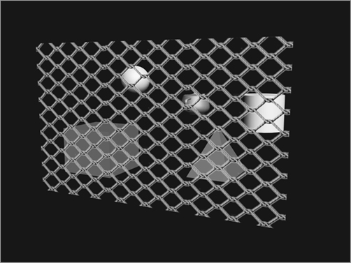
Opacity mapping allows you to cut out parts of an object by making those parts invisible. You can also create wonderful fading effects using opacity maps. With opacity mapping, you don’t have to model certain details, which can be a real time saver. In this example, you will create a chain-link fence. However, you will not model a fence. You will create it entirely from mapping. To make a chain-link fence, follow these steps:
Figure 7-83: Chain Link texture map

1. Open the Chain Link Opacity Map.max file in the Texture Scene Files folder from the companion web page. Open the Slate and from the Material/Map Browser double-click on the Standard material to add it to the view area. First you are going to add a bitmap to the diffuse color, so from the Maps ⇒ Standard rollout, double-click Bitmap and navigate to the Texture Scene Files folder from the web page. Choose Chain Link.tif (shown in Figure 7-83). This will add the Chain Link.tif bitmap node to the View Area. To link the node to the material, drag from the Bitmap output socket to the Diffuse Color input socket.
2. To make the Bitmap parameters show up, double-click on the Bitmap node. Go to the Coordinates rollout and change both the U and V Tiling parameters to 3.0. This will scale down the image across the surface of the object, because the image repeats three times.
3. Apply the material to the Plane geometry in the scene. Click the Show Standard Map in Viewport button. Render, and you will see something similar to Figure 7-84. As you can see, the chain-link image appears on the plane, but you can’t see the objects on the other side.
Figure 7-84: The chain-link fence is rendered.

4. Back in the Material/Map Browser, drag a bitmap to the Opacity input socket. This automatically links the nodes and brings up the Select Image Map File dialog box. Navigate to the Texture Scene Files folder downloaded from the web page and select Chain LinkOP.tif (Figure 7-85).
Figure 7-85: Chain Link opacity map

5. The Tiling values for the Opacity Map must be the same as for the Diffuse Map; otherwise, the transparency of the fence will not line up with the links of the fence. Double-click the opacity map node, then go to the Coordinates rollout and change both the U and V Tiling to 3.0. Render to see the results shown in Figure 7-86. Save the file.
You can see immediately how useful opacity mapping can be. 3ds Max uses the white portions of the image map to display full opacity, whereas the black areas become transparent. If you did not have an opacity file such as the one in this exercise, you could easily create one by painting a black-and-white matte of the color image that you are using for the material.
Figure 7-86: The render when both the U and V Tiling are set to 3.0
Earlier in this chapter, you turned a boring sphere into an exciting pool ball using Diffuse Color and Reflection maps. Now let’s dive into mapping the rocket we modeled in Chapter 5, “Modeling in 3ds Max: Part II,” to get it ready for lighting and rendering in Chapters 10 and 11, respectively.
To give you a rounded experience and a basis for comparison, we will use the Compact Material Editor for the following exercise, in which we create materials and map the Red Rocket model. We will then use the Slate at the end of this chapter, when we map the soldier from Chapter 6, “Character Poly Modeling.”
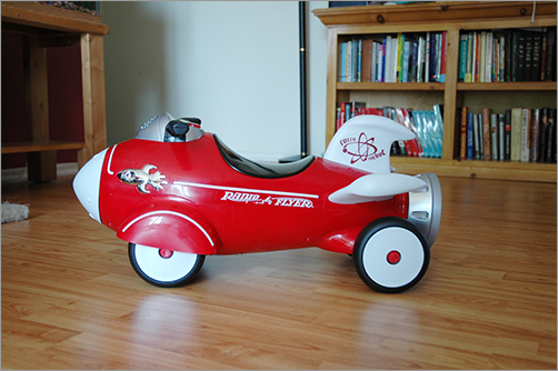
Study the full-color image of the rocket shown in Figure 7-87. (It’s also shown in the color section of this book.) That will give you an idea of how the rocket is to be textured. Let’s begin with the wheels.
Figure 7-87: Let’s texture the rocket!
The Wheels
The wheels of the real toy rocket are made of plastic that is fairly smooth, shiny, and reflective. The black tires are different from the wheels: they have a rough, bumpy surface (Figure 7-88). The bumpiness breaks up the shininess, similar to what happens when you throw a handful of sand into a pool of water. The surface is still shiny and reflective but is distorted by the bumpiness, giving an appearance of a slightly matte finish.
Figure 7-88: The tire is a rough black plastic.

Since the tire was created from a single primitive and then modified, we don’t have separate objects to which to apply materials. One option is to break apart the object so it has distinct areas (distinct objects), but this method adds an extra complication because we have to manage more objects. To avoid this, we are going to use a texturing technique using Multi/Sub-Object (MSO) materials. This material was explained earlier in the chapter; now let’s put it into practice.
Selecting Polygons and Named Selection Sets
With a Multi/Sub-Object material, you select the polygons on the objects you want to assign a particular type of material, as opposed to selecting the entire object. The hardest part of creating an MSO material is selecting those polygons. However, there are a few things that will make selecting at the sub-object level easier.
Selecting by region (see the “Selection Tool Icons” section of Chapter 3, “The 3ds Max Interface”) allows you to use the mouse to select one or more objects by defining an outline or area, instead of simply clicking them. There are five different types of regions from which to choose; the default is a rectangle region. For this task, your best bet is probably to use the Lasso region selection (which works just like the Lasso tool in Adobe Photoshop) to select the polygons around the wheel that demarcate the tire portion of the wheel.
Start by opening your final rocket model from your work in Chapter 5, or open the ROCKET_MATERIAL_WHEEL_START.max file from the Scenes folder of the Red Rocket project downloaded from the web page. This file has the rest of the rocket hidden using the Layer Manager. To unhide the other parts of the rocket, use the Layer Manager. Keep the other parts hidden for now, though.
1. Press F4 so you can see the edges on the shaded model. Press F2 so that when you select the polygons, they will be shaded and easier to see.
2. Select the wheel and go to the Polygon Modeling tab of the Graphite Modeling Tools. If the Graphite Modeling Tools don’t show up, click on the Modify tab. Select Polygon to enter Polygon Selection mode (you can also press 4 for Polygon mode).
3. Click the Select Region flyout (Figure 7-89) and select the Lasso Selection Region icon from the flyout. (Feel free to try the other region selection methods, too). Using the Lasso tool, click and drag in the viewport around the polygons you want to select to define a lasso region.
Figure 7-89: The Select Region flyout
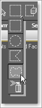
Holding down the Ctrl key lets you add polygons to your selection, and holding down the Alt key lets you remove polygons from your selection.
4. Click the Select Object tool in the Main toolbar. Then select the polygons that make up the tire portion of the wheel, as shown in Figure 7-90.
Figure 7-90: The wheel is composed of three distinct sections.

Be careful to use the Select Object tool, not the Select and Move tool. You do not want to accidentally move any of the polygons while you are trying to select them.
5. Another method to try in selecting the polygons for the black (tire) part of the wheel is to use Edge mode. Arc rotate so you are viewing the back side of the wheel. Go to Edge mode, and select a single edge on the perimeter of the wheel (Figure 7-91).
6. In the Modify Selection tab. click Loop, which will select all the edges that are touching head to toe. Then click Grow four times. Hold down the Ctrl key and click the Polygon mode.
7. Once you have selected all the tire polygons on the wheel object, as shown in Figure 7-92, save the selection as a selection set.
Figure 7-91: Select a single edge on the perimeter of the wheel.

Figure 7-92: Select all the tire polygons.

8. With the polygons selected, enter the name Wheel_Black in the Named Selection Sets field and press Enter (Figure 7-93).
Figure 7-93: Named Selection Sets field

From here on, you can select all those polygons quickly by selecting them from the Named Selection Sets pull-down menu shown in Figure 7-94.
Figure 7-94: Using named selection sets
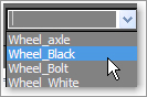
9. Once you have saved the selection set, select the white portion of the wheel, as shown in Figure 7-95 as well as in Figure 7-90. Save a named selection set called Wheel_White.
Figure 7-95: Select the white part of the wheel.

10. Finally, select the middle part of the wheel (the bolt) as called out in Figure 7-90 and shown in Figure 7-96, and create a named selection set called Wheel_Bolt.
Figure 7-96: Select the middle part of the wheel, the bolt.
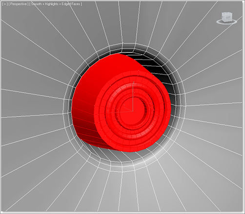
Creating a Multi/Sub-Object Material
Now that you have made your selections for the wheel, you will create the Multi/Sub-Object material for the wheel, consisting of three distinct parts: black tire, white hubcap, and red bolt.
1. Open the Compact Material Editor and select a sample sphere. We will start with the Red material for the bolt. Name the material Red Bolt, as shown in Figure 7-97.
Figure 7-97: Name the material Red Bolt.
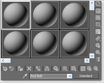
2. In the Blinn Basic Parameters rollout, select the color box next to Diffuse that controls the base color of an object; the Color Selector will open. Create a red color with the values of Red: 200, Green: 0, Blue: 0, as shown in Figure 7-98. Click Ok.
Figure 7-98: Create a red color.
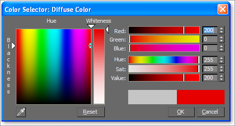
3. Change the specular highlights to make the surface appear shiny. Set the Specular Level, which controls the intensity of the highlight, to 90 and set the Glossiness, which controls the size of the highlight, to 80.
4. Select another sample sphere and set its name to Wheel White. Change the Diffuse Color to White. Set Specular Level to 90 and Glossiness to 80, as with the Red material.
5. Select a third sample sphere in the Material Editor and name it Wheel Black. Change the diffuse color to black. Because the highlights on the tire will be different, set the Specular Level to 50 and Glossiness to 20.
6. Make sure you are in Polygon mode. If the wheel bolt isn’t already selected, go to the Named Selections Set drop-down list and select Wheel_Bolt. This will select all the polygons you selected for the bolt part of the wheel.
7. Press F2 so that the selected polygons are no longer shaded full red and you can just see the edges around the poly colored red, instead. This makes it easier to see the applied material in the viewport.
8. Go to the Material Editor, select the Red Bolt material, and drag it to the selected polygons to assign it to those polygons.
9. Go to the Named Selection Sets list and choose Wheel_White, and then go to the Material Editor and grab the Wheel White material and drag it to the selected polygons, assigning the material.
10. In the Named Selection Sets list, choose Wheel_Black to select those polygons. Drag the Wheel Black material from the Material Editor to the selected polygons.
11. Your wheel now has three distinct materials applied to its appropriate parts. Save your work!
Although there are different ways to create a Multi/Sub-Object material, this method of creating an MSO material is perhaps the most straightforward and the easiest to implement in this scenario.
Loading the MSO Material into the Material Editor
Congratulations! You have created a Multi/Sub-Object material, even though it may not appear that way. What you did was create three separate materials and apply them to sub-objects on the Wheel object. What 3ds Max did was work behind the scenes to create the MSO material. How mysterious! The three materials you see in the Material Editor are now just instances of the main or parent material called the Multi Sub-Object material. We will load this material into the ME so you can see it in the following steps.
1. Exit Polygon mode by clicking on the polygon icon in the Graphite Modeling Ribbon. Open the Compact Material Editor, and select a sample sphere that isn’t being used.
2. Next to the material title is an eyedropper icon (![]() ). Click the eyedropper, and then click on the wheel. The MSO material should be loaded into the Compact Material Editor, as shown here.
). Click the eyedropper, and then click on the wheel. The MSO material should be loaded into the Compact Material Editor, as shown here.
3. The Compact Material Editor parameters for the wheel’s MSO material are shown in Figure 7-99. Change the name of the MSO material to Wheel.
Figure 7-99: The Multi/Sub-Object material for the wheel

Fine-Tuning the Materials
Continue with your own scene file. Select the Perspective viewport and press F9 for a Render Last of the wheel (F9 is the shortcut key for a Render Last). Keep in mind that the rest of the rocket is hidden and accessible through the Layer Manager.
The rendered result (shown in Figure 7-100) looks a bit flat. Specular highlights help make a 3D object look real, but highlights don’t show up on flat surfaces.
For example, in Figure 7-101, you can see three cylinder objects of varying flatness. The cylinder with the most rounded sides shows the highlight the most.
You can see a highlight on the black tire part of the wheel, but there’s no highlight anywhere on the white hubcap, and only a little highlight on the red bolt. One solution is to add more curves to your model to try to bring out the specular highlights; another solution is to change your material somehow. This decision can be made depending on how close you will see the wheel in any of your shots. If the wheel is seen only from a distance, there is no need to further detail the model. Because we will be seeing the wheel only from a distance, we will alter the material. We can add a few things to bring out the shine in the material.
Figure 7-100: The rendered wheel is a bit flat looking.
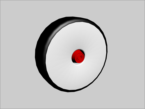
Figure 7-101: Flat objects do not show off their specular highlights particularly well.
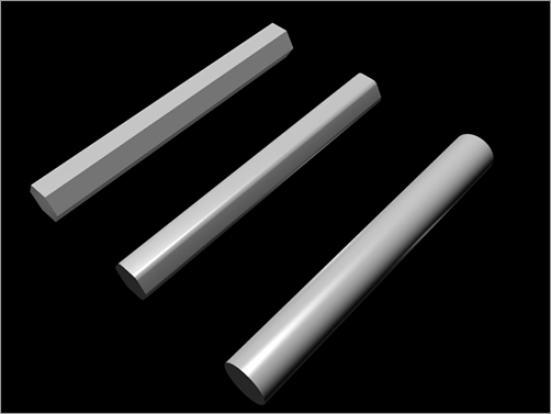
Usually shiny objects are also reflective, so if we add reflections to the flat hubcap surface, the render would look more convincing. As with the Pool Ball exercise earlier in the chapter, you can fake the reflections for a very convincing result, especially when you do not have a full CG environment built for the rocket that would allow true raytraced reflections (for more on raytracing, see Chapter 11).
To assign a reflection map to the wheel, follow these steps.
1. In the Compact Material Editor, select the Red Bolt material. In the Maps rollout, click None (to the right of Reflection). Choose Bitmap from the Material/Map Browser, navigate to the SceneAssetsImages folder in the Red Rocket project, and select the rocket Rocket Refmap Blur.jpg image file. If you don’t see this map, make sure the Files of Type field is set to JPG.
2. Render a frame of the wheel bolt. Now the wheel’s bolt will look like a perfect mirror, because the Reflection amount is being used at 100 percent.
3. In the Material Editor tools, navigate up a level (![]() ) to the Maps rollout and change the Reflection Amount to 30.
) to the Maps rollout and change the Reflection Amount to 30.
4. Repeat the preceding steps for the other two wheel materials. Figure 7-102 shows the wheel rendered with the mapped reflection. You should notice a subtle difference between Figure 7-102 and Figure 7-100, which shows the wheel with no reflections. You can adjust the Reflection Amount to taste.
The mapped reflection helps give the wheel more substance, as it makes the material more convincing when rendered. A true reflection, as you will see with raytracing in Chapter 11, will give you more accurate reflections, provided you are rendering in a created environment, which we are not. Figure 7-103 shows an example of a raytraced reflection rendered in a simple 3D room. The wheel on the left is the fake mapped reflection; the wheel on the right is the raytraced reflection showing the accurate environment.
Figure 7-102: The wheel rendered with mapped reflections

Figure 7-103: The wheel on the left has a mapped reflection, and the wheel on the right has a raytraced reflection.
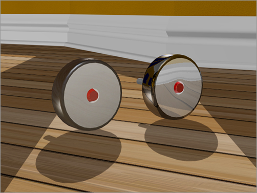
Applying a Bump Map
We are almost but not totally done with the wheel. The black part of the wheel is only halfway there. One important feature of the wheel is the bumpiness on the surface (refer to Figure 7-88 earlier in the chapter). This bumpiness changes all the specular and reflective properties on that part of the wheel. Bump mapping is very common in CG. It adds a level of detail to an object fairly easily by creating bumps and grooves in the surface and giving the object a tactile element. Bump mapping uses the intensity values (aka the brightness values) of an image or procedural map to simulate bumpiness on the surface of the model, without changing the actual topology of the model itself. You can create some surface texture with a bump map; however, you will not be able to create extreme depth in the model. For that, you may want to model the surface depth manually or use displacement mapping instead. To add a bump map to the tire, follow these steps:
1. In the Compact Material Editor, you should have the Wheel Black material selected and the Maps rollout open from the previous series of steps.
2. Click the None button next to the Bump map. In the Material/Map Browser, choose Noise.
Noise is a map of color patterns that is generated procedurally in three dimensions so you don’t have to fuss with mapping coordinates. (Mapping coordinates specify the location of an image on your object, as discussed later in the chapter.)
Figure 7-104: Noise Parameters rollout

3. When you place the Noise map in the Bump map slot, you will automatically be taken to the Parameters for the Noise map in the Compact Material Editor (Figure 7-104). Change the Size to 0.02. Click the Go to Parent icon (![]() ) to move up a level to the main Material parameters.
) to move up a level to the main Material parameters.
4. Go to the Maps rollout and increase the Bump Amount from 30 (the default) to 60.
5. Render; you should now see a texture on the tire (Figure 7-105) that resembles the real bumpiness of the tire in Figure 7-88.
The wheel is complete!
Now you’ll need to apply the MSO material you created to the other three wheels. There’s a hard way to do this, and an easy way. The hard way is to select the polygons for the tire, the hubcap, and the bolt for each wheel, and apply the MSO material. The easy way is to copy the finished wheel, place it where the other three wheels are located, and delete the original wheels. Just make sure to unhide the rest of the rocket using the Layer Manager.
Figure 7-105: Add a bump map to the wheel.

Creating Material Libraries
While a material is in the Material Editor or applied to an object, it is part of the scene and is saved with the scene, whether it is displayed in a sample slot in the Material Editor or not. However, for complicated scenes it is inconvenient to have all the materials active in the Material Editor, because you are limited to only 24 sample slots. Once you get to your 25th material, you will have to store some of the materials elsewhere, such as in a Material Library, to make available slots for editing in the Material Editor. You can later bring those stored materials back into the Material Editor easily.
To create a Material Library, follow these steps:
Figure 7-106: The Material/Map Browser options menu
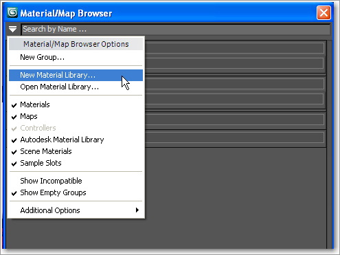
1. In the Compact or Slate Material Editor, select the Material node or sample sphere with the Wheel Multi/Sub-Object material.
2. Click on the Get Material button in the Compact Material Editor (![]() ).
).
3. In the Material/Map Browser, click on the Options button (![]() ), which is in the upper-left corner. This opens the menu shown in Figure 7-106.
), which is in the upper-left corner. This opens the menu shown in Figure 7-106.
4. Choose New Material Library from menu and name the Library Red Rocket (Figure 7-107).
Figure 7-107: Name the library Red Rocket.
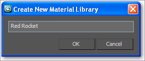
5. Now the Material/Map Browser has a rollout, Red Rocket. Drag and drop the MSO material (and any other material from your scene) from the Material Editor to the Material/Map Browser’s Red Rocket rollout. This automatically loads it into the Red Rocket library.
6. To save the library to a location to be used at another time, right-click on the Red Rocket title bar; you will see the path it is set up in. Choose Save As (Figure 7-108).
Figure 7-108: Save the Red Rocket library.
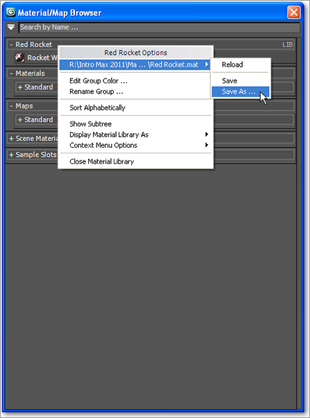
7. Save the Library in the MaterialLibraries folder in the Red Rocket project. Name it Red Rocket.mat. (There already is a file in that folder called ROCKET.mat for your reference.)
You can also load a library from a 3ds Max scene file, instead of a Material Library file (.mat). When you click Open Material Library from the Material/Map Browser’s option menu, choose Open Material Library and then choose 3ds Max (*.max) from Files of Type. Select and load the .max scene file. All materials assigned in that scene are then listed in the browser. To convert the collection of materials to a library file, click Save and save it as a MAT file (.mat).
You can load the scene file ROCKET_MATERIAL_WHEEL_FINAL.max from the Scenes folder of the Red Rocket project on the web page to skip to this point or to check your work.
Mapping the Fins: Introduction to Mapping Coordinates
An image map is two-dimensional; it has length and width but no depth. Geometry in 3ds Max, however, extends in all three axes. How is a material that contains 2D image maps applied properly to a 3D scene object? Are the maps projected in a single direction onto the object’s surfaces or do they envelop the object cylindrically or spherically? The answer depends on the type of mapping coordinates applied to the object. Mapping coordinates define how and where image maps are projected onto an object’s surfaces and whether the maps are repeated across those surfaces.
Mapping coordinates can be applied to objects in several ways. The Generate Mapping Coords option is on by default. When primitive objects are created and the Generate Mapping Coords option is checked at the bottom of the Parameters rollout, the appropriate mapping coordinates are created automatically.
Loft objects, which are covered in Chapter 5, control mapping in the Mapping section of the Surface Parameters rollout. The Length Repeat value determines how many times the material’s maps are repeated along the length of the Path object, and the Width Repeat value determines how many times the maps are repeated around the scene object.
If any part of your rocket is hidden in the scene file, especially if you started with the scene files from the web page, unhide those parts in the Layer Manager.
The Base Material
The top vertical fin on the rocket’s tail is nothing special as far as materials are concerned. It is white plastic that is just a bit shiny and has a decal, as you can see in Figure 7-109. At this point, you easily can create the material itself:
1. Open the ROCKET_MATERIAL_FIN_START.max file from the Scenes folder of the Red Rocket project, and continue with the ROCKET_MATERIAL_WHEEL_FINAL.max or the file you have created.
2. Open the Compact Material Editor and select an available sample sphere. In the Blinn Basic Parameters, click the color swatch next to the Diffuse, and make it white.
3. Name the material Fin_Decal. Unlike the side fins, the top fin has a decal on its side, so it will have its own material. Apply the material to the Fin object by dragging and dropping the sample sphere from the Material Editor to the fin.
4. Back in the Material Editor, in the Specular Highlights group of the Basic Blinn Parameters set the Specular Level to 80 and the Glossiness to 60. When you render, the base color may look a bit gray; that is just the basic lighting in the scene. See Figure 7-110.
Figure 7-109: The top vertical fin of the rocket
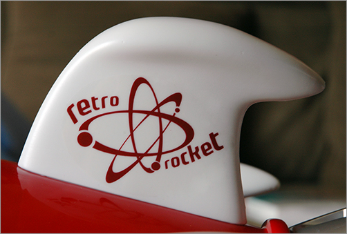
5. We need to add reflections for the fin. Go to the Maps rollout in the Material Editor, click None next to the Reflection map, and select Bitmap from the Material/Map Browser. Navigate to the SceneAssetsImages folder in the Red Rocket project and select Rocket Refmap Blur.jpg to assign it as the reflection map.
6. The Compact Material Editor will display the Bitmap Parameters rollout. Go up a level by clicking on the Go to Parent icon. Go to the Maps rollout and turn the Reflection Amount down to 35.
7. Render. You’ll see a plain, white, shiny fin, as shown in Figure 7-111.
Figure 7-110: Fin with basic material applied
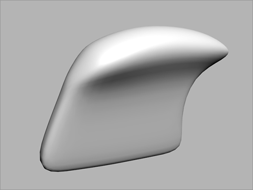
Figure 7-111: Turn the Reflection amount down to 35 to achieve this render.
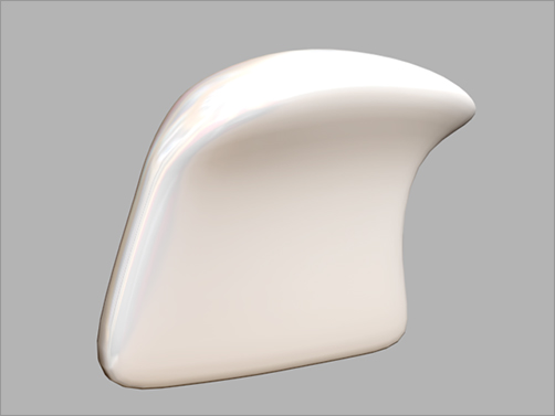
Adding the Decal
The main feature of this vertical fin is its decal. This is an image that we need to add to the material. The image is a 2D image and won’t be as easy to apply as the 3D noise map we used earlier for the bump map of the tire. The decal will become a part of the Diffuse color; we will replace the color we created for Diffuse with the image itself.
1. In the Compact Material Editor, select the Fin_Decal sample sphere. Make sure you are at the top level of the material and can see the Maps rollout.
2. Click None next to the Diffuse Color map. Choose Bitmap from the Material/Map Browser, navigate to the SceneAssetsImages folder in the Red Rocket project, and choose RedRocketDecal.tif.
3. In the Material Editor toolbar, click the Show Standard Map in Viewport button (![]() ). This will display the decal in the viewport. Figure 7-112 shows the mapped decal on the top fin.
). This will display the decal in the viewport. Figure 7-112 shows the mapped decal on the top fin.
Figure 7-112: The decal isn’t mapping properly to the top fin.
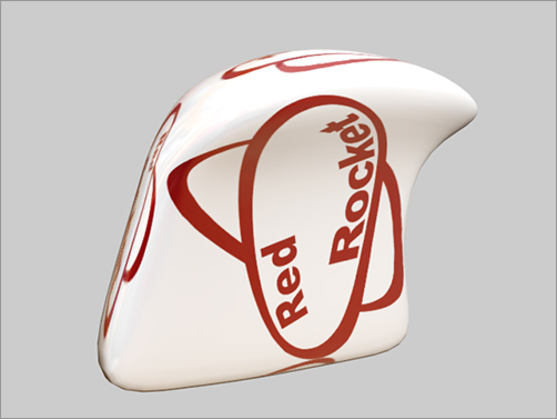
Don’t panic just yet. Every object in 3ds Max has a set of mapping coordinates that tell the program how to place a 2D image onto your geometry. Honestly, 3ds Max gets it wrong most of the time the first time you try to map a 2D image.
4. In the Material Editor’s parameters for the decal, go to the Coordinates rollout (shown in Figure 7-113); this area is where you adjust the map. Details about the parameters in this section are discussed in the “Coordinates Rollout Explanation” sidebar.
5. The decal needs to be rotated, scaled, and positioned. In the Material Editor, under the Coordinates rollout, change Angle W to 90.
Figure 7-113: The Coordinates rollout for the bitmap parameters

6. Set the Tiling to U: 1.6 and V: 2. With bitmap coordinates, the higher the number, the smaller the map will become, in order to allow it to repeat or tile. In this case, we do not want the bitmap to repeat; we’re just using the values to shrink the size of the decal on the surface. To turn off the tiling, simply uncheck the Tile boxes.
7. Set the Offset to U: –0.11 and V: 0.05.
The size and placement of the decal are not bad, but there are still copies of the decal on all the sides of the top fin, as shown in Figure 7-114.
This happened because the model for the top fin started out as a box with six sides, so the Material Editor put a decal on each side of the geometry. This method works if the bitmap image has a random pattern and you don’t mind having that image on all sides of the object. Here, the mapping coordinates inherent in the top fin geometry will not allow us to place the decal on just the sides of the fin.
In the next section, we will use a modifier to change the mapping coordinates on the Top Fin object.
Figure 7-114: Copies of the decal are still on all sides of the top fin.
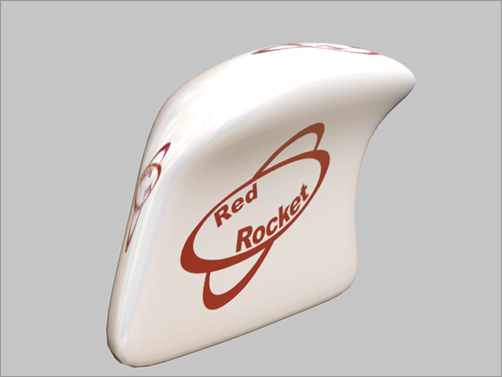
Coordinates Rollout Explanation
The Coordinates rollout in the bitmap parameters for a 2D image has several options, as you can see in Figure 7-113. Here is a brief explanation of the settings:
Applies the map as a texture map or environment You can select the type of coordinates from the Mapping pull-down menu. As you can see in Figure 7-113, there are different coordinate choices for Textures or Environments.
Offset UV Changes the position of the map over the surface of the geometry. U moves the bitmap horizontally, and V moves the bitmap vertically on the surface.
Tiling UV Determines the number of times the map is repeated along each axis.
Angle UVW Rotates the map about the U-, V-, or W-axis in degrees.
Using a UVW Mapping Modifier
Instead of dealing with the surface’s own mapping coordinates as we have been doing, we are going to use a modifier to replace those coordinates on the geometry. The UVW Mapping modifier makes the decal act more like a real decal that we can control by moving a modifier gizmo around to place the coordinates as we please. (For more on UVW mapping, see the sidebar “Understanding UVW Mapping” later in this chapter.)
The UVW Mapping modifier is commonly used to apply and control mapping coordinates. You select the type of mapping projection, regardless of the shape of the object, and then set the amount of tiling in the modifier’s parameters. The mapping coordinates applied through the UVW Mapping modifier override any other mapping coordinates applied to an object, and the Tiling values set for the modifier are multiplied by the Tiling value set in the assigned material. Figure 7-115 shows the parameters for the UVW Mapping modifier.
Figure 7-115: The UVW Mapping modifier’s parameters
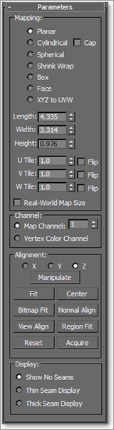
Creating the UVW Mapping Modifier
To use the UVW Mapping modifier to properly map the decal to the fin, follow these steps.
1. Go back to the Compact Material Editor and set the coordinates in the bitmap parameters for the decal back to their default values:
Offset: U: 0.0, V: 0.0
Tiling: U: 1.0, V: 1.0
Angle: W: 0.0
UV Tile boxes: Check Off to turn the Tiling feature off
2. Select the fin and go to the Modify panel. From the Modifier List drop-down, choose UVW Mapping.
3. In the Modifier Stack, you can see the UVW Mapping modifier stacked on top of the Editable Poly. You will also see an orange gizmo next to the top fin geometry.
When you apply the UVW Mapping modifier to your object, the gizmo always conforms to the shape of the object. Because this is a decal, we want the image to keep its original proportions.
4. Go to the UVW Mapping modifier parameters and, in the Alignment section, click the Bitmap Fit button (shown in Figure 7-116).
Figure 7-116: The Alignment section for the UVW Mapping modifier parameters
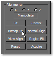
5. This will take you to the Select Image dialog box. Navigate to the SceneAssetsImages folder in the Red Rocket project and select the file RedRocktDecal.tif. This will change the size of the UVW Mapping gizmo to the size and aspect of the image rather than the geometry.
Adjusting the UVW Mapping Gizmo
Now we will adjust the UVW Mapping Gizmo in the following steps:
1. In the Modifier Stack, click the plus sign in the black box next to the UVW Mapping modifier, and select Gizmo. See Figure 7-117.
Figure 7-117: Select the sub-object Gizmo mode for the UVW Mapping modifier.

2. Now look at the top fin in the viewport, and you should see the plane-shaped Modifier gizmo. You will now be able to transform it to suit where you need the decal placed.
3. Switch to the Rotate tool, and rotate 75 degrees on the X-axis.
4. Switch to the Scale tool (press R), and scale down the gizmo to 40 percent. Then switch to the Move tool (W) and center the decal on the fin as shown in Figure 7-118.
5. In the viewport, the decal looks like a bright white rectangle, while the rest of the top fin is gray. That is okay. Render, and you will see something similar to Figure 7-119.
Figure 7-118: Center the decal on the fin.
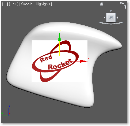
Figure 7-119: Render, and the decal will look much better on the fin.
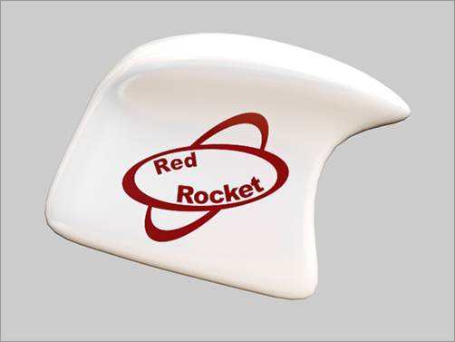
Correcting the Projection
While the decal on this side of the fin looks fine, if you look on the other side of the fin, the decal is flipped. The type of UVW Mapping modifier projection we are using (planar mapping) is useful only when one side of an object needs to be mapped. In this case we need the decal to show up correctly on the other side of the fin. What do we do now?!?
Figure 7-120: The decal shows in places we don’t want.

1. Go to the UVW Mapping modifier parameters, and select Box under Mapping.
2. This works, but now we have the decal in places we don’t want, as shown in Figure 7-120. This is because Box mapping projects the image from six sides, using a planar map for each side, but uses the sided-surface normal (a vector that defines which way a face or vertex is pointing) to decide the mapping direction. So, we are going to trick the modifier and remove the depth.
3. In the parameters for the UVW Mapping modifier, change the Height parameter to 0.01, as shown in Figure 7-121.
Figure 7-121: Change the Height parameter to 0.01.
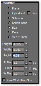
4. The copies of the decals we don’t want on the fin should disappear. On the sides where we don’t want the decal, we have scaled the Box Projection gizmo down to almost nothing; the projections for those sides are actually still there but now they are very small and not noticeable on the fin. This isn’t the most sophisticated way to fix the issue, but it works for our needs. In CG, whatever works is the best course of action. See Figure 7-122 for final results.
We can’t change the Height parameter of the UVW Mapping modifier gizmo to 0 because then the modifier won’t work properly. A very small value such as 0.01 works very well instead.
Figure 7-122: Fin with final materials
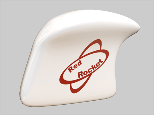
Adding the Material to the Material Library
This is a good time to add this decal material to the Material Library.
1. Select the Fin_Decal material in the Material Editor and click the Get Material button (![]() ).
).
2. In the Material/Map Browser, go to the Material/Map Browser Option button (![]() ). Choose Open Material Library and navigate to the MaterialLibraries folder in the Red Rocket project.
). Choose Open Material Library and navigate to the MaterialLibraries folder in the Red Rocket project.
3. Choose the file Red Rocket.mat from the MaterialLibraries folder. Then drag the Fin_Decal material from the Material Editor to the Red Rocket library in the Material/Map Browser.
4. Right-click on the Red Rocket title bar and choose the path and save.
5. Render out the fin and check your work. Save your scene file.
You can load the scene file ROCKET_MATERIAL_FIN_FINAL.max in the Scenes folder of the Red Rocket project to skip to this point or to check your work.
Understanding UVW Mapping
The UVW Mapping modifier consists primarily of a yellow gizmo that determines how the image maps are projected onto the surfaces of an object. The images are projected outward or inward from the gizmo and extend through the assigned objects to all surfaces. The size and orientation of the gizmos affect how the maps are projected onto the relevant objects. The properties of the different mapping types are listed here:
Planar Projects the image map perpendicular to the perimeter of the rectangular gizmo.
Cylindrical Projects the map outward from the center of a cylindrical gizmo as if the map were wrapped around the object in two axes.
Cap Projects the map to the end caps of the cylindrical gizmo in a planar fashion.
Spherical Projects the map outward from the center of a spherical gizmo as if the map were completely enveloping the object. The top and bottom of the image maps are gathered at the poles of the gizmo and may cause some distortion.
Shrink Wrap Similar to the Spherical method, except that the four corners of the image map are gathered at a single location.
Box Projects the image in six perpendicular planes from the center of the gizmo.
Face Applies the image map to each face of an object regardless of its size or orientation.
XYZ to UVW Used with procedural maps, such as Noise or Smoke, to control the maps when the object changes size.
Mapping the Body
The rocket body is made up of three texturing areas:
The main body: red with a white decal
The control panel: a gray metallic material
The nose: white plastic with teardrop embossed features
The easiest way to texture is to use the Multi/Sub-Object material technique you used on the wheel. The body has a logo on it, so it will have the same issue as the fin: The logo image will appear on the opposite side of the object when you use Planar mapping. Another way of dealing with the logo-flipping issue is to apply the material to each side separately. You would apply the same material to specific selected polygons on each side of the object, but 3ds Max lets you apply two maps and two UVW Mapping modifiers instead of one. This gives you independent control over each side of the rocket body.
This is the technique you would use if you wanted to put a different design on the other side of your model.
Figure 7-123: Select Ignore Backfacing

1. Open the ROCKET_MATERIAL_BODY_START.max.
2. Select the rocket and go to the modeling ribbon. Go to Polygon mode and select the polygons on one half of the rocket. This is accomplished most easily in the Top viewport.
The Seat and Control panel polygons are also selected now. We want to deselect them for now. To do this, go to the modeling ribbon, and under Polygon Modeling select Ignore Backfacing; see Figure 7-123.
Figure 7-124: Select one half of the rocket’s body, without the seat or control panel polygons.
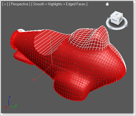
This allows you to select only the polygons facing you. Hold down Alt while you select what you want to subtract from any selection. This can be a bit tedious, but it must be done. Once finished, your selection should resemble Figure 7-124.
Creating the Material
We’ll begin by creating a material for the red body.
1. Open the Compact Material Editor, select a sample sphere, and click on the color swatch next to Diffuse. Change the color to red (with values of R: 200, G: 0, B: 0). Name the material Rocket Body Right.
2. Drag and drop the new material onto the selected polygons of the rocket to assign the material to that half of the rocket.
3. Go to the Maps rollout and click on None next to Diffuse Color. Choose Bitmap from the Material/Map Browser and navigate to the SceneAssetsImages folder in the Red Rocket project and select the file ![]() ). Don’t worry if the map doesn’t look correct.
). Don’t worry if the map doesn’t look correct.
4. Use the Go to Parent button in the Material Editors toolbar and navigate to the top level of the material. In the Specular Highlights section of the Material Editor, change the Specular Level to 90 and Glossiness to 80.
5. Go to the Maps rollout and click None next to Reflection, and from the Material/Map Browser choose Bitmap. Navigate to the SceneAssetsImages folder in the Red Rocket project and select the file Rocket Refmap blur.jpg for the reflection. Go back to the Maps rollout and change the Amount value next to Reflections to 20.
6. Press the F9 key to do a Render Last. The decal will probably be tilting (Figure 7-125), so we see part of it toward the front and the seat of the rocket.
Figure 7-125: The decal is tilting.
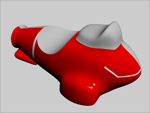
7. Go back to the Material Editor, and in the Coordinates rollout uncheck the Tile UV boxes to turn off tiling. Don’t worry if the map doesn’t look quite right yet. The map on the rocket may appear in a strange layout, such as shown previously, or may even be a strange color (in some rare cases).
The model still needs mapping coordinates. We will get to them later.
Flipping the Decal
In the following steps, we will create a copy of the one side’s material and flip it for the other side.
1. Go back to the modeling ribbon, and select the polygons on the opposite side of the rocket. Remember to deselect the Seat and Control panel polygons.
2. In the Compact Material Editor, drag and drop the Rocket Body Right material sample sphere onto an available sample sphere to make a copy of the material. Rename the material Rocket Body Left.
3. Go to the Maps rollout for this new material and click the button next to Diffuse Color to take you to the bitmap parameters. Click the bar with the image path and, in the file selection window, select RocketBodyLeft.tif for a flipped version of the previous color map.
Figure 7-126: Change to Map Channel 2 in the Coordinates rollout of the bitmap.

4. In the Coordinates rollout, change the Map Channel parameter to 2, as shown in Figure 7-126. This lets you have many different sets of coordinates on the same object simultaneously. Don’t worry that the Red Rocket graphic disappears; it will return when we add the UVW Mapping modifier for the left of the rocket.
5. Drag and drop the flipped material onto the selected polygons of the rocket (representing the other side of the rocket).
We are now adding the mapping coordinates. We have two materials for each side of the rocket. The right side of the rocket has Map Channel 1 and the left side has Map Channel 2. We are going to start by adding and editing the mapping for the right side with Map Channel 1.
Figure 7-127: Change to X in Alignment parameters of the UVW Mapping modifier.
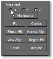
6. Go into the Modify panel and click the Editable Poly entry to leave the sub-object selection level. Then, from the Modifier List, choose the UVW Mapping modifier. We are going to keep it on the default mapping setting, which is Planar. In the Alignment parameters of the modifier change to the X-axis, as shown in Figure 7-127.
7. Click the Bitmap Fit button, navigate to the SceneAssetsImages folder in the Red Rocket project, and select the file RocketBodyRight.tif. This will change the Modifier gizmo to make it the same size as the bitmap image, keeping the image’s scale proportional.
8. In the Modify panel, go to the Modifier Stack and click on the black box with the plus sign next to the UVW Mapping modifier. Click on Gizmo to allow you to transform the image (via the gizmo) without affecting the object.
9. Move the Modifier gizmo so the white stripe in the decal is lined up approximately with the front of the rocket, as shown in Figure 7-128.
10. Exit the UVW Mapping modifier gizmo sub-object mode by clicking the modifier in the stack.
Figure 7-128: Line up the stripe in the material just like the real rocket’s stripe.

11. Add a second UVW Mapping modifier onto the rocket, and change the Map Channel to 2 (Figure 7-129).
Figure 7-129: Select Map Channel 2 in the UVW Mapping modifier.
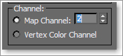
12. In the Alignment parameters of the second UVW Mapping modifier, change the axis to X. Click on the Bitmap Fit button, navigate to where the RocketBodyLeft.tif bitmap is found, and click Open.
13. Go to the Modifier Stack, click the Gizmo sub-object, and move the bitmap gizmo to line up the image with the map on the opposite side of the rocket.
If you render, you should now see the stripe decals on the side of the rocket, as shown in Figure 7-130.
Figure 7-130: A render of the rocket shows how the decal is mapped on the body.

Adding a Seat
Figure 7-131: Adding the seat

We don’t have to worry about mapping the polygons of the seat for the rocket because we have a model of a seat to add.
Go to the Application menu and choose Import ⇒ Merge, navigate to the Scenes folder in the Red Rocket project, and select the file SEAT.max and click Open to merge in the seat geometry, as shown in Figure 7-131. The extra geometry adds detail to the model by giving it a nicer seat. If you had to, you could forgo the seat geometry, instead selecting the seat polygons and assigning a glossy black material to them.
The control panel and Nose materials still need to be created and added to the model.
The Control Panel
In this section, we will texture the control panel.
1. As you have done before, create a new material in an available sample sphere in the Material Editor and set its color to gray. If you prefer, you can just use the default gray (R150, G150, B150).
2. Set the Specular Level to 50 and the Glossiness to 20.
3. Name this new material Control Panel.
For the control panel, we should add just a little bit of bumpiness to the surface to give the panel a better feel.
4. Select the Control Panel material in the Material Editor. In the Maps rollout, change the Bump Amount to 20 and click None to create a map.
5. Select Noise from the Material/Map Browser to add a Noise texture to the bump map.
6. In the Noise Parameters rollout for the Noise map, change the Size to 0.02.
Finally, let’s add a reflection map to the control panel, as we did with the body of the rocket.
7. In the Material Editor, click Go to Parent, then select the Maps rollout, set the Reflection Amount to 10, and click None next to Reflection to add a map.
8. Select Bitmap from the Material/Map Browser and navigate to the Red Rocket project’s SceneAssetsImages folder to select Rocket Refmap blur.tif.
9. In a viewport, select the rocket, enter Polygon mode, and select the polygons that make up the control panel, as shown in highlight in Figure 7-132. Drag the Control Panel material onto the selected polygons to assign the material.
Figure 7-132: Select the polygons of the control panel.

10. Click on the Editable Poly level when you are finished. If you don’t, the two UVW Mapping modifiers will be applied only to the control panel polygons.
Because the buttons of the control panel are separate objects, you easily can create colorful materials for them, using more or less the same settings from the previous materials. Simply assign each button its own material for its own distinctive color. If you are using ROCKET_MATERIAL_BODY_START.max, the finished control panel buttons are hidden in their own layer. Open the Manage Layer dialog box and unhide the layer.
Voilà! All that remains now are the thruster and the nose of the rocket.
Bring on the Nose, Bring on the Funk
The material for the nose is pretty similar to the material we just created for the control panel, except the Diffuse color should be white.
1. Copy the Control Panel material by dragging it onto an empty sample sphere in the Compact Material Editor and changing its Diffuse color to white. Feel free to adjust the Specular settings as you see fit. (A Specular level of 90 and a Glossiness value of 80 work very well.) Name the new material Nose.
The control panel had a slight bump map on the material. Let’s remove that from the Nose material.
Figure 7-133: Clear the Bump bitmap.

2. Select the Nose material in the Compact Material Editor. Right-click on the map bar next to the Bump parameter, and select Clear from the context menu, as shown in Figure 7-133.
The Nose material now has no bump map, but it retains the reflection map from the control panel’s material, saving us a little bit of work.
3. Select the polygons of the nose, shown in a box in Figure 7-134, and drag the material from the Material Editor to the selected polygons to assign the material. When you’re finished, click Editable Poly to return to object mode.
Figure 7-134: Select the polygons of the nose.

4. Save your work, and make sure to version up the file as not to overwrite your previous scene file. The Rocket’s side decals will look wrong until you click the top UVW Mapping modifier.
The Thruster
The final part of the rocket model to texture is the thruster. Using the experience you’ve already gained from texturing the rest of the rocket, this will be a breeze. If you prefer, you can load the ROCKET_MATERIAL_THRUSTER_START.max file from the Scenes folder of the Red Rocket project, or just continue with your own scene.
Figure 7-135 shows the thruster. Notice the round bulbous section in the left image. This is the middle yellow part of the thruster.
In this section, we’ll experiment with a selection technique to make it easier to isolate the middle, yellow part of the thruster. Also remember to use the Layer Manager to unhide any parts of the rocket that may be hidden in your scene.
1. Select the thruster and enter Polygon mode. Select the center ring of polygons of the thruster, highlighted in Figure 7-136.
If the Thruster object is not an editable polygon in your scene, add an Edit Poly modifier to the object before continuing.
2. In the modeling ribbon, in the Modify Selection tab, click the Grow button five times to enlarge your selection to include all the polygons that make up the yellow round inside of the thruster, highlighted in Figure 7-137.
3. Open the Material Editor and select an available sample sphere. Name this material Thruster Yellow Light. If there are no available sample slots, right-click on a slot and choose 5 × 3 Sample Slots from the menu.
4. In the Blinn Basic Parameters rollout, click on the color swatch next to Diffuse and change the color to yellow (R: 255, G: 210, and B: 0).
5. In the Specular Highlights section, change Specular Level to 90 and Glossiness to 80.
6. To give the yellow material a bit of a lightness, change Self Illumination to 50 and Opacity to 90.
Figure 7-135: The Thruster object has a yellow part, the circle in the middle, and the outside housing.

Figure 7-136: Select the center ring of polygons of the thruster.

Figure 7-137: Click the Grow button in the Modify Selection tab.

7. Go to the Maps rollout and change the Reflection Amount to 50 and add a bitmap to Reflection. Navigate to the SceneAssetsImages folder in the Red Rocket project and select the file Rocket Refmap blur.tif to add a reflection map similar to the rest of the rocket.
8. Drag and drop the material to the selected polygons.
9. To save a lot of time, we can easily select the other polygons of the thruster. With the round center polygons still selected, choose Edit ⇒ Select Invert.
10. Drag and Drop the Control_Panel material onto the selected polygons. Done! Figure 7-138 shows the textured thruster.
11. Unhide all the other parts of the rocket using the Layer Manager, as needed, and render a frame of the fully textured rocket, as shown in Figure 7-139 and Figure 7-140.
All the parts of the rocket now have materials applied.
Save your work, pat yourself on the back, and have a nice smoothie to celebrate. All the parts of the rocket now have materials applied.
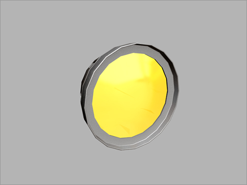
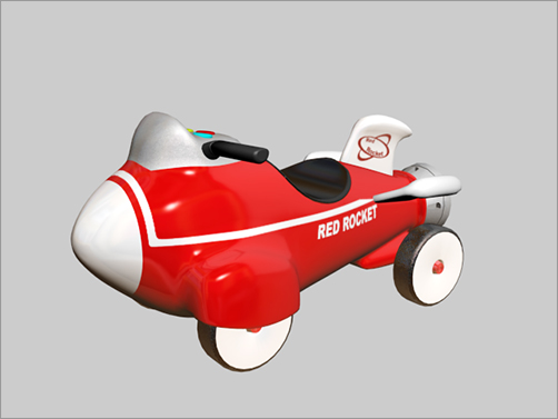
Figure 7-140: The rocket from behind
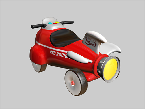
In this exercise, we will apply materials and maps to the soldier model from Chapter 6. For this process, we will first UV unwrap the model so we can lay out the colors and patterns for the soldier’s uniform and general look. This process essentially creates a flat map that can be used to paint the textures in a program such as Photoshop. Having properly laid out UVs will make the mapping process much easier.
We have already created the textures (i.e., the maps) we intend to use for the soldier using Adobe Photoshop.
The remainder of this chapter will show you how to prepare the model for proper UVs and how to apply the maps we have already painted. We will not be showing the actual painting process in Photoshop, as it goes beyond the purposes of this book.
UV Unwrapping
Set your project to the Soldier project downloaded from the companion web page at www.sybex.com/go/intro3dsmax2011. Open the scene file SoldierTexture_v01.max from the scenes folder of the project, or use your own final model scene file from Chapter 6. Keep in mind that any design changes you made to your own soldier model may cause discrepancies in the UV unwrapping and mapping steps completed in the following sections.
In this section, we will unwrap the UVs for the soldier model by creating seams on the soldier’s body that will define body shapes on a flat blank canvas that can be used later for painting the textures for those parts of the body. For example, we will begin by creating seams to define the shapes of the arms, so we know where in Photoshop to paint the sleeves of the uniform.
Begin defining UVs with the following steps:
1. Turn on Smooth + Highlights + Edged Faces view for your viewports.
2. With your model selected, go to the Modifier List drop-down panel and add an Unwrap UVW modifier to it, as shown in Figure 7-141.
Figure 7-141: Add an Unwrap UVW modifier.

3. Expand the Unwrap UVW modifier in the Modifier Stack and enter into Face mode, as shown in Figure 7-142.
4. Turn off Show Map Seam under the Parameters rollout. This turns off the green highlight on the edges, which is generated by default and is not useful in its current state.
5. Click the Point to Point Seam button toward the bottom of the Command panel under the Map Parameters rollout (Figure 7-143). This tool will let us re-route the seams to where we want them.
Figure 7-142: Enter into Face mode.

Figure 7-143: Click the Point to Point Seam button.
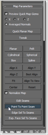
6. With Point to Point Seam enabled, click on the center of a pair of intersecting edges about where you want to define the left shoulder (Figure 7-144). A dashed line “rubber band” appears next to your cursor, letting you know that the tool is waiting for the next point to be selected.
7. Select the next intersecting edges in the loop around the shoulder. This creates a blue highlight across the edges (see Figure 7-145).
Figure 7-144: Pick this edge intersection to begin defining the left shoulder.
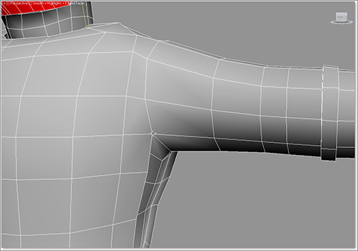
Navigating Viewports while Point to Point Seam is Active
While Point to Point Seam is active, you can navigate using all the viewport navigation tools to look around the model. After you’ve done so, 3ds Max still remembers the last intersection you clicked and draws an accurate seam at the next click.
8. Continue around the shoulder until you have a complete loop, ending with the intersection you started with in step 6. Also, you can right-click then start or continue the picks without overlapping the picks.
9. Select the bottom-most edge intersection on the underarm and continue selecting edge intersections all the way to the middle point of the wrist, as shown in Figure 7-146. You will have to switch to Wireframe (press F3) view to pick the last point (Figure 7-147) at the end of the forearm.
10. Click the right mouse button to deactivate the Point to Point Seam tool’s rubber banding, but still keep the button active, then continue cutting a new set of UVs for the right arm as you did for the left arm.
11. Right-click the mouse, and box out areas under the arms on both sides as shown in Figure 7-148. In Figure 7-148, you can see the seams block out the area under the arm and continue down to the belt line, and across the top of the beltline around the waist. If you miss-click a point, you can use the Undo button.
Figure 7-145: Pick these edge intersections.

Figure 7-146: Select the intersections under the arm.

Figure 7-147: Switch to Wireframe view to pick the last intersection for the forearm/wrist.

Figure 7-148: Add these seams to define the torso areas under the arm.

12. Using the Point to Point Seam tool, cut seams for the two gloves lengthwise down the middle from wrist to wrist. You can see this progression for the left-hand glove start in Figure 7-149. Begin at the wrist on the side of the thumb and work your way around to the opposite side of the wrist. Remember, you may need to enter Wireframe view mode (F3) to select the proper edge intersection points. Figure 7-150 shows the seam working around the hand.
13. Open the Material Editor (Slate or Compact) and apply an unused Standard material to your entire model if it doesn’t already have one. Double-click on the Diffuse Color input socket of the material (Figure 7-151) to open the Material/Map Browser (Figure 7-152). Under the Maps ⇒ Standard rollout, select Checker and click OK.
14. In the Slate, double-click the Checker Map title bar to open its parameters. Change the U and V Tiling parameters for the checker map from 1 to 5 so the checker texture (Figure 7-153) gives you better visual feedback as to how your UVs are coming along as you fix them. At the top of the Slate, click on Show Standard Map in Viewport if you cannot see the map on your model in the viewports (Figure 7-154).
Figure 7-149: Cut a new seam along the glove, starting as shown.
Figure 7-150: Work your way around the glove.
Figure 7-151: Double-click the Diffuse Color input socket.
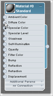
Figure 7-152: Double-click to create a Checker map for the diffuse color.

Figure 7-153: Set the U and V Tiling to 5.
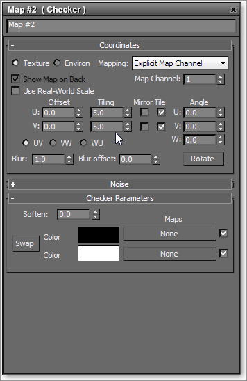
Figure 7-154: Click the Show Standard Map in Viewport button.
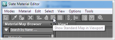
Pelting the Left Arm UVs
Save your work now before continuing with the next set of steps to unfold the UVs for the arms into usable patterns to paint the textures. You can pick up with the scene file SoldierTexture_v02.max from the Scenes folder of the Soldier project from the companion web page to check your work so far or to skip to this point.
1. With Face mode selected in your Unwrap UVW modifier, and Point to Point Seam unselected, click on a polygon on the left forearm of your model. Next, in the Command Panel at the bottom of the Map Parameter rollout, click on the Exp. Face Sel to Seams button. If the seams were created correctly in the previous set of steps, a selection of faces on the arm will turn red in your viewport (Figure 7-155).
2. Now we need to unfold the UVs to create the pattern to paint on in Photoshop (or another image editor). To unfold the UVs into a usable pattern, click on the Pelt button in the Map Parameters rollout, as shown in Figure 7-156.
3. When you click Pelt, 3ds Max opens the Edit UVWs dialog box as well as the Pelt Map dialog box. In the Edit UVWs dialog box, click the View menu and check off Show Grid and Show Map to simplify the UV view as shown in Figure 7-157.
Figure 7-155: The arm’s faces are selected.
Figure 7-156: Click on Pelt to unfold the UVs of the arm.
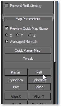
Figure 7-157: The Edit UVWs and Pelt Map dialog boxes showing the arm UVs
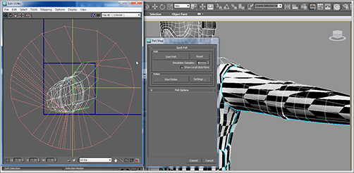
4. To unfold the map, click on the Start Pelt button in the Pelt Map dialog box. This moves the UVs in the Edit UVWs dialog box in real time. This procedure keeps unfolding the UVs until you stop it, so wait a couple of seconds for the UVs to stop moving, and click on Stop Pelt. Figure 7-158 shows the results.
Figure 7-158: Pelting the arm UVs

Figure 7-159: Set the drop-down menu to Relax by Face Angles.

5. You’re almost done with the arm, but if you check the checkerboard texture in your viewport you can see that some of the checks are bigger than others. To fix this, click the Settings box next to the Relax button in the Pelt Map dialog box, and change the drop-down option to Relax by Face Angles (Figure 7-159). Click the Set as Default button since you will be going through these steps on each part of your model.
6. Now, click on Start Relax. Wait until the UVs stop moving and click on Stop Relax. Checking your texture in the viewport now shows the checkerboard how we want it (Figure 7-160).
7. In the Pelt Map dialog box, click on the Commit button at the bottom, or your changes won’t take. Also, you want to exit out of the Edit UVWs dialog.
Figure 7-160: The arm UVs are pelted and relaxed the way we need them.
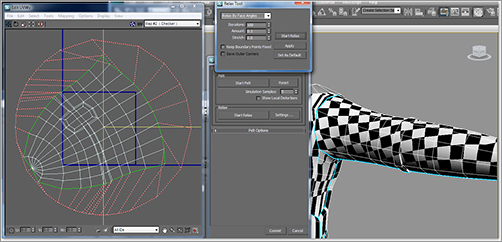
Pelting the Right Arm UVs
Repeat Steps 1–7 for the right arm. You can see in Figure 7-161 that the right arm is now laid out—pelted and relaxed.
Figure 7-161: The right arm is pelted and relaxed.
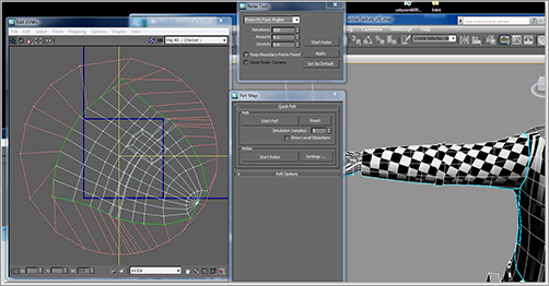
Unwrapping and Using Pelt for the Head
Save your work now before continuing with the next set of steps to unfold the UVs for the head. You can pick up with the scene file SoldierTexture_v03.max from the Scenes folder of the Soldier project downloaded from the companion web page to check your work so far or to skip to this point.
For this section, since it is a bit hard to see where to seam, we went into the Material Editor to the Standard Checker material we created. In the Maps rollout, we unchecked Diffuse Color to turn off the checker pattern.
The head poses a problem: Each part (helmet, goggles, mask) is a separate object modeled in Chapter 6 that was attached together into one Editable Polygon. That means when we look closely at the geometry, there is some object penetration. This makes it very hard to clearly see some of the areas we need to seam. We will use a sub-object visibility technique to control what we are viewing in the following steps.
1. Select the Soldier, and in the Modify panel’s Modifier Stack, go to Editable Poly, and select Element, as shown in Figure 7-162. Element mode allows you to select separate objects that are attached together into a single object.
Figure 7-162: Go into Element mode to select the helmet.

When you do this you will get the warning shown in Figure 7-163. Select Yes. Every time you move between the Unwrap UVW modifier and the Editable Poly modifier, you will see this warning; if that gets annoying, check the Do Not Show This Message Again option. The warning tells you that any changes you make to that level of the model will ripple throughout the rest of the stack and may mess up other parts of your work. Since we are simply using the Element mode to hide parts of the head of the model to make seaming easier to see, we need not worry that anything will change.
Figure 7-163: Topology dependency warning
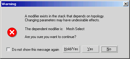
2. Select the helmet, then in the modeling ribbon go to the Visibility tab and click Hide Unselected, as shown in Figure 7-164. That this will hide all unselected elements in the model, leaving the helmet as the only visible object. Yay!
Figure 7-164: Hide Unselected hides all the elements except the helmet.
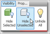
3. Exit Element mode by clicking Editable Poly in the Modifier Stack. Now go back up to the Unwrap UVW modifier and click on Face. Go back down to the Map Parameters rollout and click the Point to Point Seam button. Following the line in Figure 7-165, create a new seam on the helmet.
4. When the seam is has been created, go back down to the Editable Poly ⇒ Element mode in the Modifier Stack, and in the Visibility tab click the Unhide All button. Then select the goggles, go to the Visibility tab, and click Hide Unselected button. Repeat step 3 on the Goggles using Figure 7-166 as your guide for the seams.
Figure 7-165: Create a new seam on the helmet.

Figure 7-166: Goggle guide for the seams
5. Repeat the process individually for the mask, the head, and the helmet straps, using Hide Unselected to isolate each of the three elements as you work on them. Then follow the same process as before to create seams as shown in Figure 7-167 for the face mask, Figure 7-168 for the head, and Figure 7-169 for the helmet strap.
6. Open the Material Editor, and in the soldier’s checker material go to the Maps rollout and check the box next to Diffuse Color to turn on the checkers again. We will need the checkers when we pelt the model.
Figure 7-167: Seams for soldier face mask

Figure 7-168: Seams for the soldier head
Figure 7-169: Seams for the soldier helmet strap

Seaming the Rest of the Body
Use the Point to Point Seam tool to block out the rest of the model’s parts and then pelt map them as you did for the arms. Refer to Figures 7-170 and 7-171 for the placement of seams on the model’s body. These figures are also shown in the color section of this book.
Figure 7-170: Follow these outlines to create the rest of the model’s seams. This image is also in the color section of this book.
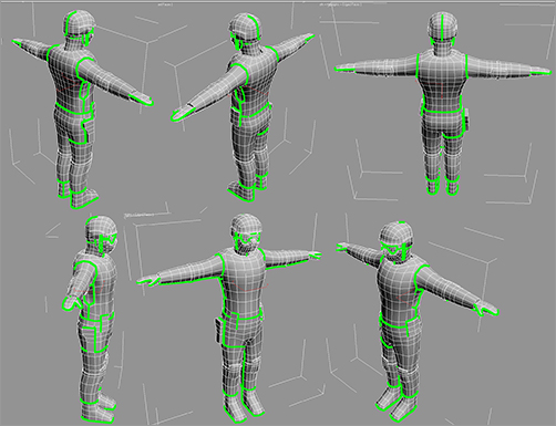
Unfolding the Rest of the Body
Save your work before continuing with the next set of steps. You can pick up with the scene file SoldierTexture_v04.max from the Scenes folder of the Soldier project downloaded from the companion web page to check your work so far or to skip to this point.
1. In the Modify Panel, click the Face button. Then click a single polygon on the helmet. Then select the Exp. Face Sel to Seams. This will select all the polygons associated with the seams you created for the helmet.
Figure 7-171: Follow these outlines to create the rest of the model’s seams for your model. This image is also in the book’s color section.
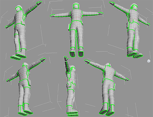
2. Click the Pelt button. This will open the Edit UVWs dialog box and the Pelt Map dialog box. First click Start Pelt. You will see the UVs moving around; when they stop moving, click the Stop Pelt button.
3. Now click on the Settings button next to the Start Relax button. Make sure the drop-down menu is set to Relax by Face Angles and click the Save as Default button. Then exit out of the Relax Tool dialog box.
4. Click the Start Relax button again, and when the UVs stop moving, click Stop Relax. For the remaining objects you don’t have to go into the settings box: Just hit Start Relax.
5. Select the Commit button. The checkers pattern on the helmet should look organized and even.
Now that you are finished with the helmet, make your way down the body using Pelt and Relax to lay out the UVs on the remaining parts of the body, checking each one off as you go.
Save your work now before continuing with the next set of steps. You can pick up with the scene file SoldierTexture_v05.max from the Scenes folder of the Soldier project to check your work so far or to skip to this point.
As you can see in Figure 7-172, when the UVs are finished, the checker pattern for each separate part of the soldier is a different size.
1. In the Modify panel, click the Face button if it isn’t already selected. Then click away from the Soldier model and drag a selection box around the whole model to select all the polygons as shown in Figure 7-172.
Figure 7-172: Soldier model with all the polygons selected

2. Under the Parameters rollout in the Unwrap UVW modifier click the Edit button. What you will see is a mess; these are all the unwrapped UVs piled on top of each other.
3. In the Edit UVWs menu, go into Tools ⇒ Relax. Click Start Relax. Be patient and wait for the movement to slow down or stop before pressing Stop Relax. Then exit out of the Relax Tool dialog box. This will relax all of your UVs together uniformly, ensuring that they all have the same UV real estate. This is important so that all the elements carry the same relative texture space as each other, as shown in Figure 7-173.
4. Keep the Edit UVWs dialog open. Deselect the UVs by clicking away from the model. You should see what is shown in Figure 7-174.
Figure 7-173: Soldier model with all UVs relaxed uniformly

Figure 7-174: The Edit UVWs dialog box with the soldier UVs in a pile

Because you are still in Face mode in the Unwrap UVW modifier, if you click anywhere on the pile of UVs you will select a face. What we want to do now is to select an individual e element’s full set of UVs so that we can lay them out separately, giving them some space on the flat blank canvas that can be used later for painting the textures for those parts of the body. The easiest way is to select a face, then go down to the toolbar at the bottom of the Edit UVWs dialog box and check Select Element, as shown in Figure 7-175.
Figure 7-175: Check Select Element.
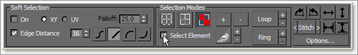
This will allow you to select all the UVs associated with an element (such as the helmet only). When you select something in the Edit UVWs dialog box it will show up selected on the model in the viewports, as shown in Figure 7-176. This will help you know what parts you are moving around in the Edit UVWs dialog. Also in the Edit UVWs dialog box you can use all the navigation tools you use in the viewports to pan and zoom. In the following steps, you will start placing the UVs for each element within the thick blue bordered box in the Edit UVWs dialog box to lay out the entire soldier’s UVs for textures.
1. In the Edit UVWs dialog box, drag a selection box around all the UVs. Using the Scale tool in the Edit UVW dialog box, scale the UVs about -25%. Now you should be able to see the blue border box in the Edit UVWs dialog box, as shown in Figure 7-177.
Figure 7-176: Select an element in the Edit UVWs dialog box, and it will show as selected on the model.
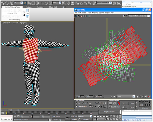
Figure 7-177: Scale down the UVs until they fit in the blue box.

Figure 7-178: UVs correctly placed within the UV space. This image is also included in this book’s color section.

2. Click on the Select Element option, then start moving and rotating the elements to separate each element’s UV layout from the others by selecting the UV points and moving them within the blue box to eventually match the layout in Figure 7-178. Figure 7-178 is also shown in the color section of the book for clarity. The goal is to fit the UVs into this box without going outside of it, and without overlapping any of the UVs. Anything outside this box will end up tiling (or have no texture at all), and any overlapping UVs will share parts of the texture from another element. Either way, that’s not good.
3. If you find that there simply isn’t enough room to fit all of the UVs in, select all the UVs again, and scale them down together uniformly as you did in Step 1, and continue placement. Figure 7-178 shows the UVs laid out and correctly placed within the usable UV space.
4. In the Edit UVWs dialog, select Tools ⇒ Render UV Template to open the Render UVs dialog box shown in Figure 7-179. In that dialog, click the Render UV Template button to create an image of your UVs, as shown in the Render Map dialog box in Figure 7-180.
5. Save the UV layout image by clicking the Save Image icon in the Render Map dialog box (Figure 7-181). Once saved, this image can be opened in your favorite image editor and you can use the pieces as guides to paint the soldier’s textures.
Figure 7-179: Render UVs dialog box
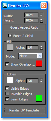
Figure 7-180: The UV rendered image

Figure 7-181: Save the UV image.
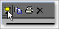
With the UV layout image saved, you can go into Photoshop (or image editing software of your choice) and create a texture to place on your model. The UV image was taken into Photoshop and with a combination of painting and cutting/pasting of photos, the final map for the soldier was created (Figure 7-182). Figure 7-182 is also in the color insert of this book.
The texture map, as you can see, places painted parts of the soldier’s body according to the UV layout we just created. For example, you can clearly see the soldier’s vest painted in the upper-left corner of the texture image file, with the back of the vest in the upper part, the neck hole in the middle, and the front of the vest below.
The more you unwrap UVs for models, the easier it becomes to anticipate how to paint the textures. Unwrapping a human character model like this soldier, even a simple model like this, is not an easy affair, but is the cornerstone to successfully creating good looking assets for games or animations.
Figure 7-182: The final map for the soldier.
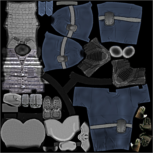
In the following sections, we will show you how to apply the maps to the material for the soldier, as well as explore bump and normal maps to give the soldier added detail.
Applying the Color Map
Save your work now before continuing with the next set of steps. You can pick up with the scene file SoldierTexture_v06.max from the Scenes folder of the Soldier project to check your work so far or to skip to this point.
Now it is time to use the map we put so much effort into.
1. Open the Slate. You should see the checker material we created for the soldier to help with the UVs. Drag a Standard material from the Material/Map Browser to the view area. Name it Soldier.
2. Double-click on the Diffuse Color input socket of the material to open the Material/Map Browser. Under the Maps ⇒ Standard rollout, select Bitmap. When the Select Bitmap Image File dialog box appears, navigate to the /SceneAssets/images folder for the Soldier project, and select the Soldier_Color_V04.tif file.
3. Apply the material to the soldier and click on Show Standard Map in Viewport; the result is shown in Figure 7-183. BAM! Now wasn’t all that hard UV work worth it?
Figure 7-183: The soldier with the material applied.

Applying the Bump Maps
Bump mapping makes an object appear to have a bumpy or irregular surface by simulating surface delineation. When you render an object with a bump-mapped material, lighter (whiter) areas of the map appear to be raised on the object’s surface, and darker (blacker) areas appear to be lower on the object’s surface, as shown in Figure 7-184.
Normal mapping is a technique used for faking the lighting of bumps and dents. It is used to add details without using more polygons in the modeling process. A Normal map is usually used to fake high-resolution geometry detail while it’s actually mapped onto a low-resolution mesh for efficiency’s sake. The pixels of a normal map each store a vector (or simply, a direction) that describes a high resolution surface’s slope at that very point on the surface. This vector is called a normal. The RGB channels of a normal map control the direction of each pixel’s normal, enabling you to fake a high degree of surface resolution when applied to a low polygon mesh. A normal map for the soldier is shown in Figure 7-185 and in the color section of the book.
Figure 7-184: Bump map created in Photoshop by desaturating the original color map to create light and dark areas that conform to the original color texture
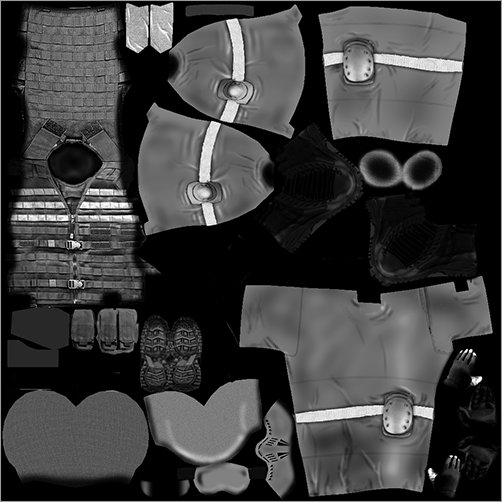
Figure 7-185: Normal map created in Photoshop and based on the original color map. This image is also included in the book’s color section.

You can use one or both of these mapping techniques to create additional surface detail. It all depends on how much detail you want to appear. Bump maps are simpler to create, since you can usually take the color map and just desaturate it to make a grayscale image file. Normal maps are not as simple but yield better results when the object is rendered. We have both a normal map and bump map for you to use. We will continue with the Soldier material we created in the previous exercise as we add these new maps in the following steps.
1. Click on the Bump input socket of the material to open the Material/Map Browser. Under the Maps ⇒ Standard rollout, select Normal Bump.
Figure 7-186: The Normal Bump node’s Parameters rollout
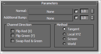
2. Click on the title bar of the Normal Bump node to bring up the Parameters rollout shown in Figure 7-186. Click on the None button next to Normal. This will once again bring up the Material/Map Browser. Under the Maps ⇒ Standard rollout, select Bitmap. When the Select Bitmap Image File dialog box appears, navigate to the /SceneAssets/images folder of the Soldier project, and select the Soldier_Normal_V01.tif file.
3. Back to the Normal Map Parameters: now click None next to Additional Bump. This will once again bring up the Material/Map Browser. Under the Maps ⇒ Standard rollout, select Bitmap. When the Select Bitmap Image File dialog box appears, navigate to the /SceneAssets/images folder from the Soldier project downloaded from the companion web page, and select the Soldier_BS_V01.tif file.
4. Go back to the Maps rollout in the main material parameters and set the Bump Amount to 100.
The Normal map is applied and finished. See Figure 7-187 for the material tree from the Slate. See Figure 7-188 for images that compare the soldier rendered with and without the Normal map. Figure 7-188’s images are also shown in the book’s color section. You may notice that the normal and bump maps have created a lot more detail in the soldier’s body, particularly in his vest. You should notice the difference even better in your own renders.
Figure 7-187: The Slate Material Editor node tree with a Diffuse Color map and a Bump map

Figure 7-188: The left image is a render of the soldier without the Normal and Bump maps. The right image is rendered with the Bump/Normal maps.

Applying the Specular Maps
Highlights in objects are actually a reflection of a light source, and specularity is a way to fake those reflections by placing highlights on the receiving surface that would otherwise be reflecting the light in reality. Specular maps are maps you use to define a surface’s shininess and highlight color, without the complex calculations of actual reflections in the render. The higher a pixel’s value (from black to white, or 0 to 1 respectively), the shinier the surface will appear at that location. Therefore, dry matte surfaces such as unpolished stone or fabric would have a very dark specular map, while polished surfaces like shiny metal or glossy plastic would have lighter specular maps.
We will be adding a specular map to the soldier to further the amount of detail we can get from the render. We are going to reuse the image that we used for the Bump map to give the soldier a bit of bling on his vest and buckles.
In the Slate, drag from the output socket of the Additional Bump bitmap to the Specular Level input socket of the Soldier material already in your scene, as shown in Figure 7-189.
The final render of the soldier is shown in Figure 7-190 as well as in the color section of the book. You can notice the improvement to the look of the soldier’s vest with the added Specular Color map.
Now your soldier character is ready to use in renders, or even as a game asset. There are many online resources on how to export assets such as the soldier to your favorite game engine. We will use the soldier for rigging and animation with Character Studio in Chapter 9, “Character Studio and IK Animation,” as well as use him for rendering exercises in Chapter 11.
Figure 7-189: Dragging from the Bump map to the Specular slot.

Figure 7-190: Final render of the soldier

Creating materials for your objects is usually the next step after modeling them. Creating materials can give you a sense of accomplishment because it is essentially the last step in making the object look as you envisioned—aside from lighting and rendering, of course.
There are several ways to create materials, from simple colors to complex mappings on distinct parameters. Finding the right combination of maps, shader types, and material types can make a world of difference in the look of your scenes. It’s important to remember that like everything else in CG, applying materials takes time, and gaining wisdom with your materials and maps will come with practice.
In this chapter, you learned the basics of materials, what kinds of materials are in 3ds Max, and how to create and edit them in the Material Editor. Then you learned how choosing the appropriate type of shader will make your surface look right, and how to apply your knowledge to mapping a pool ball, reflections and all. Next you learned a few more tricks with the Material Editor and found out about the different kinds of maps available in 3ds Max. With that knowledge, you mapped the entire rocket you modeled in Chapter 5, and readied it for its next step, lighting in Chapter 10. Then you picked up the soldier model from Chapter 6 and learned how to lay out its UVs for painted textures, which you assigned at the end of the chapter using color as well as bump, normal, and specular maps.
If you’d like some additional practice, go back and adjust all the materials on the rocket with different types of materials, colors, and settings to see how they affect the render of the rocket. So far we’ve done all this with a minimal lighting setup. As you will see in Chapter 10, lighting plays a vital role in how you texture your model. Soon you’ll find yourself tweaking settings for the specular highlights, reflections, color, and so on as you change your lighting environment to create the best render.