
Chapter 5
It’s a Matter of Demand and Supply
In This Chapter
![]() Learning the basics about the demand–supply model
Learning the basics about the demand–supply model
![]() How exchange rates are determined based on the demand–supply model
How exchange rates are determined based on the demand–supply model
![]() Which factors change exchange rates
Which factors change exchange rates
You may know today’s dollar–euro exchange rate, but it will be something else tomorrow or the next day. Why do exchange rates change? Reading this chapter is the first step in answering this question.
Economists don’t use a crystal ball to predict changes, although some people may think so! But economists have a pretty nice set of tools at their disposal for prediction. This chapter shows that the demand–supply framework enables you to predict the next period’s exchange rate. When you understand this framework, you’ll be able to predict the direction of the change in the exchange rate — in other words, whether a currency will depreciate or appreciate against another currency.
This chapter introduces a basic microeconomic approach to exchange rate determination. First, the market for oranges illustrates the demand–supply model. Then you can easily change the assumption from the market for oranges to the market for dollars or euros.
Apples per Orange, Euros per Dollar: It’s All the Same
Think about a barter economy that uses no money and in which people exchange oranges for apples. Basically, in the orange market, some people do have a demand for oranges. Other people produce oranges and supply them to the market. People who have apples are prepared to exchange them for oranges at a certain price. Producers of oranges are also prepared to exchange oranges for apples at a certain price.
This section develops a demand–supply model that determines the price and quantity of oranges in the market.
Price and quantity of oranges
In this barter economy, we exchange apples for oranges, and vice versa. Therefore, the amount of apples necessary to buy one orange is the price of an orange (in apples). Figure 5-1 shows the orange market.

Figure 5-1: Market for oranges.
In Figure 5-1, the x-axis indicates the quantity of oranges. Moving to the right on the x-axis, the quantity of oranges in the market increases. Moving to the left on the x-axis, the quantity of oranges in the market decreases. The y-axis measures the price of oranges. As you move up on the y-axis, the price of an orange increases; it means that you give up more apples to buy one orange. As you move down on the y-axis, the price of orange decreases; it means that you give up fewer apples to buy one orange.
Demand and supply in the orange market
In microeconomic analysis, the market for a good, in this case, the market for oranges, is shown by the demand and supply curves. The demand curve represents the consumers’ demand for oranges. The negative slope of the demand curve implies that as the price of oranges increases, the quantity demanded of oranges declines, and vice versa. The supply curve shows the behavior of orange producers. The positive slope of the supply curve indicates that as the price of oranges increases, orange producers supply a higher quantity of oranges, and vice versa.
Figure 5-1 illustrates the demand for and supply of oranges. The intersection of the demand and supply curves indicates the market price and quantity of oranges. Another term for the market price and quantity of oranges is the equilibrium price and quantity of oranges. In this example, the market price of oranges is 2 apples, which means that consumers give up 2 apples to buy an orange, and producers receive 2 apples when they sell an orange.
The equilibrium price and quantity of oranges doesn’t stay the same, so you want to predict the changes in the price and quantity of oranges in the market. If any changes occur in the factors that affect either the supply or the demand curve, the equilibrium price and quantity of oranges changes.
In economics jargon, these factors are called ceteris paribus conditions (meaning “everything else constant”). The assumption is that the values of these factors are fixed along the demand and supply curves. When they change, the curve shifts in the appropriate direction.
Assume that the latest medical research indicates that oranges cure cancer. The demand for oranges then rises. As Figure 5-2 shows, an increase in the demand for oranges increases the price and quantity of oranges in the market.
Now assume that excessive cold destroyed most of the orange harvest in the U.S. In this case, the supply curve declines. Figure 5-3 shows that a decline in the supply curve increases the price of oranges and decreases the quantity of oranges in the market.

Figure 5-2: Orange consumption cures cancer and changes the market price of oranges.

Figure 5-3: Cold weather damages the orange harvest and changes the market price of oranges.
These changes can occur simultaneously. As you see in Figure 5-4, if the demand curve increases thanks to the incredible health benefits of oranges and the supply curve decreases because of cold weather, the price of oranges will increase. In Figure 5-4, the price of oranges increases to 2.5 apples per orange. But the effect on quantity is undetermined. Figure 5-4 shows one of the three possible outcomes in terms of quantity and assumes no change in the quantity of oranges because the increase in the demand curve is the same as the decline in the supply curve.
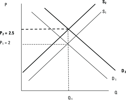
Figure 5-4: Oranges cure cancer, cold weather damages the orange harvest, and the orange price increases in the market.
Of course, you can change your assumptions regarding the nature of the shocks affecting the orange market. This time, assume harmful properties of oranges to health (oranges cause cancer) and, at the same time, the introduction of a disease-resistant variety of orange trees. In this case, the demand curve declines and the supply curve increases, lowering the market price of oranges with an undetermined output effect.
In the next section, this demand–supply approach is applied to exchange rate determination.
Determining Exchange Rates through Supply and Demand
Keep the following in mind when applying the demand–supply model to exchange rates:
![]() An exchange rate implies the relative price of a currency. For example, the euro–dollar exchange rate tells you how many euros to give up to buy one dollar. Therefore, this exchange rate implies the price of a dollar in euros. If the exchange rate is expressed as the dollar–euro rate, it tells you how many dollars to give up to buy one euro. Therefore, this exchange rate implies the price of a euro in dollars.
An exchange rate implies the relative price of a currency. For example, the euro–dollar exchange rate tells you how many euros to give up to buy one dollar. Therefore, this exchange rate implies the price of a dollar in euros. If the exchange rate is expressed as the dollar–euro rate, it tells you how many dollars to give up to buy one euro. Therefore, this exchange rate implies the price of a euro in dollars.
![]() Certain forces affect the demand for and supply of dollars, or of any other currency, in foreign exchange markets. Because exchange rates are the main subject here, this section identifies which factors affect the demand and supply of currencies.
Certain forces affect the demand for and supply of dollars, or of any other currency, in foreign exchange markets. Because exchange rates are the main subject here, this section identifies which factors affect the demand and supply of currencies.
![]() The demand–supply model of exchange rate determination implies that the equilibrium exchange rate changes when the factors that affect the demand and supply conditions change.
The demand–supply model of exchange rate determination implies that the equilibrium exchange rate changes when the factors that affect the demand and supply conditions change.
This section uses the market for dollars as an example, but you can use any market you want. (The last section of this chapter assumes the market for euros.) Whichever market you use, be careful when labeling the x- and y-axes of your model. When in doubt, remember the setup in the orange market. If you have the quantity of oranges on the x-axis, you have to put the price of oranges on the y-axis. Then the supply and demand curves inside the model refer to oranges.
Also, think about the meaning of the demand for and supply of dollars. Who are these people that want to buy or sell dollars or any other currency? I discuss them in Chapter 3. They are international banks, multinational companies, speculators, and so on. Whenever they want to buy dollars, they’ll be along the demand curve. Whenever they want to sell dollars, they’ll be along the supply curve.
Let’s apply this discussion to the dollar market.
Price and quantity
If you want to graph the dollar market, the quantity on the x-axis must be the quantity of dollars in the market. Therefore, the price indicated by the y-axis must be the price of dollars in another currency (in this example, the euro). In other words, the exchange rate has to be defined as the euro–dollar exchange rate. Consequently, the demand and supply curves indicate the demand for and supply of dollars. Figure 5-5 shows the initial equilibrium exchange rate as €0.89 per dollar.
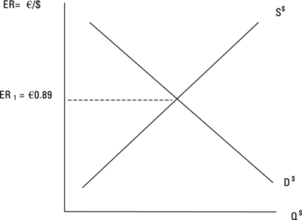
Figure 5-5: Market for U.S. dollars.
 Even though this chapter talks about the demand and supply of dollars, don’t think about the “domestic” money demand and supply. In terms of exchange rate determination, the domestic money market becomes important in Chapters 6 and 7. For now, think about foreign exchange markets where market participants buy or sell currencies for the reasons explained in the next section.
Also note that Figure 5-5 and the following figures focus on the changes in the exchange rate and don’t indicate the changes in the quantity of currency in question.
Factors that affect demand and supply
As in the case of the demand and supply curves in the orange market, ceteris paribus conditions are associated with the demand and supply of dollars. These conditions are related to the macroeconomic fundamentals of two countries represented in the exchange rate.
Because the example exchange rate is the euro–dollar rate, the following variables may change in the U.S. or the Euro-zone, which then have an effect on the euro–dollar exchange rate:
![]() Inflation rate
Inflation rate
![]() Growth rate
Growth rate
![]() Interest rate
Interest rate
![]() Government restrictions
Government restrictions
In the demand–supply model, these factors are divided into two areas based on how they affect exchange rates. Inflation rate and growth rate are considered trade-related factors. When you apply the changes in one of these factors to exchange rates, you think about the trade between the U.S. and the Euro-zone.
The interest rate, on the other hand, is a portfolio flow–related factor. It means that when one of the country’s interest rate changes, you think about how this change affects the attractiveness of dollar- and euro-denominated securities to American and European investors.
Government restrictions can be related to both trade flows and portfolio flows, depending on the nature of these restrictions.
 Note that the changes in inflation, growth, and interest rates, as well as government restrictions, don’t have to be actual changes that you are observing right now. If market participants have expectations regarding these changes, they will act on them now, producing the same results as if these changes were actually happening.
Predicting Changes in the Euro–Dollar Exchange Rate
In this section, a change in each of the macroeconomic fundamentals (inflation rate, growth rate, interest rate, and government restrictions) is applied to the dollar market.
Inflation rate
The demand–supply model predicts that the higher-inflation country’s currency will depreciate. Continuing with the U.S. and the Euro-zone example, if the U.S. has a higher inflation rate than that of the Euro-zone, the dollar is expected to depreciate against the euro. Following is the explanation for this prediction.
 When you work with the demand–supply model of exchange rate determination, first think about whether the relevant factor is related to trade or portfolio flows. Second, think about the people represented by the demand and supply curve and what they would do, given the nature of the change in one of the macroeconomic fundamentals.
Remember that inflation rate is a trade-related variable. If the U.S. inflation rate is higher than that of the Euro-zone, at the given exchange rate, European goods become less expensive to American consumers. Therefore, Americans are inclined to sell their dollars, buy euros, and buy European goods. This increases the supply of dollars in the market.
However, at the given exchange rate, American goods become more expensive to European consumers because of higher inflation rates in the U.S. Therefore, European consumers are now less inclined to buy American goods. Their demand for dollars decreases. Figure 5-6 indicates these shifts.
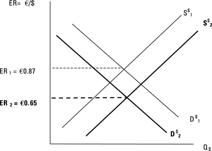
Figure 5-6: The U.S. inflation rate increases.
Figure 5-6 shows that the dollar depreciates (and the euro appreciates) when the U.S. runs a higher inflation rate than the Euro-zone.
Growth rate
Economic growth refers to an increase in a country’s output, or real gross domestic product (real GDP). The demand–supply model predicts that the higher growth rate country’s currency will depreciate. For example, if the Euro-zone’s real GDP growth rate is higher than that of the U.S., this model predicts that the euro will depreciate.
All other predictions of the demand–supply model are consistent with the monetary approach to exchange rates introduced in Chapters 6 and 7. Growth rate of real GDP is the only factor about which different theories provide different predictions. In upcoming chapters, the currency of the country with the higher growth rate will appreciate.
For simplicity, assume that the U.S. growth rate shows no change and the Euro-zone’s growth rate increases. Again, remember that growth rate is a trade-related variable. If the Euro-zone’s growth rate is higher, then at the given exchange rate, Euro-zone’s consumers and businesses are expected to buy more consumption and investment goods from the U.S. Therefore, Europeans are inclined to sell their euros, buy dollars, and buy American goods. As Figure 5-7 shows, this increases the demand for dollars and the price of dollars, which leads to the appreciation of the dollar (or the depreciation of the euro).

Figure 5-7: The Euro-zone’s growth rate increases.
Interest rate
Remember, interest rate is a portfolio flow–related factor. Think of yourself as an investor who is deciding between a dollar- and a euro-denominated investment opportunity (with the same risk). Because the main subject is portfolio investment, the interest rate considered here is the real interest rate.
The real interest rate is defined as the difference between the nominal interest rate and the inflation rate (see Chapter 4).
This model predicts that the currency of the country with the higher real interest rate will appreciate. As an investor, and at the given exchange rate, you decide to invest in a security that gives you a higher real return. Suppose that the Euro-zone’s real interest rates are higher. Figure 5-8 shows the implications of this change on the euro–dollar exchange rate.

Figure 5-8: The Euro-zone’s real interest rate increases.
When you look at the demand and supply curve in Figure 5-8, identify the investors along these curves. As the real interest rate on Euro-denominated securities increases, investors’ demand for dollar-denominated securities declines. Therefore, the demand for the dollar declines. In terms of the supply of dollars, investors are inclined to sell their dollars in exchange for euros to buy euro-denominated securities. As Figure 5-8 shows, the supply curve for dollars increases. Both an increase in the supply curve and a decrease in the demand curve lead to the appreciation of the euro (or the depreciation of the dollar).
Government interventions
Assuming that trade and portfolio flows aren’t restricted, domestic consumers and investors have a choice of which country’s goods to consume and which country’s currency to invest in. However, governments may be concerned about this freedom and may not like domestic consumers’ and investors’ demand for foreign goods or portfolios.
The previous exercises in this chapter explain why governments may feel this way. Favoring foreign goods and portfolios implies the exchange of the domestic currency for foreign currency, which depreciates the domestic currency. Therefore, sometimes governments implement restrictions on trade or portfolio flows to prevent the domestic currency from further depreciation. These restrictions are expected to appreciate the restriction-imposing country’s currency.
Suppose that the U.S. starts imposing tariffs on some of the European Union’s (EU) imports. To keep the exercise simple, assume that the EU doesn’t retaliate. Figure 5-9 shows that trade restrictions imposed by the U.S. lead to a decline in the supply of dollars. The reason is that trade restrictions are prompting U.S. consumers to exchange fewer dollars for euros. The result is the appreciation of the dollar (or the depreciation of the euro).
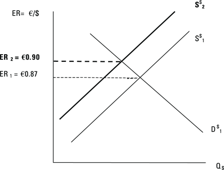
Figure 5-9: The U.S. implements restrictions on European imports.
Figure 5-9 also illustrates government restrictions on capital flows. If the U.S. imposes restrictions on portfolio outflows, U.S. investors exchange fewer dollars for euros to put in a euro-denominated deposit. Therefore, the supply of dollars declines, and the dollar appreciates (and the euro depreciates).
Keeping It Straight: Using a Different Exchange Rate
You can repeat the entire analysis in the previous section using a different exchange rate. For example, we can invert the euro–dollar exchange rate, which implies the price of the dollar in euros. Now you have the dollar–euro exchange rate, which implies the price of a euro in dollars.
Since the price of a euro is given, on the x-axis of the model, you need to consider the quantity of euros. This time, the demand and supply curves indicate the demand for and supply of euros, which makes it the market for euros.
Figure 5-10 indicates this change. Note that the equilibrium exchange rate is the inverse of the euro–dollar rate of €0.87, or approximately $1.15 (1 ÷ 0.87).
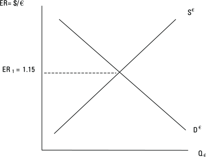
Figure 5-10: Market for euros.
You can apply the same shocks that we applied to the dollar market, this time to the euro market. You’ll be shifting different curves, but you should come to the same predictions in terms of the change in the exchange rate.
Take the increase in the U.S. inflation rate. Your argument remains the same. At the given exchange rate, American consumers will buy more goods from the Euro-zone countries, and Euro-zone consumers buy fewer goods from the U.S. Therefore, the demand for the euro increases and the supply declines, which increases the dollar–euro exchange rate. This situation shows a depreciation of the dollar (or an appreciation of the euro).
If the Euro-zone’s real GDP growth rate is higher than that of the U.S., at the given exchange rate, European consumers buy more American goods. This scenario also increases the supply of euros and appreciates the dollar (or depreciates the euro).
If the real interest rate in the Euro-zone is rising, investors increase their demand for euro-denominated securities and, therefore, the euro, which then increases the demand curve for euros. With higher real interest rates on euro-denominated securities, investors sell fewer euro-denominated assets and, therefore, sell fewer euros, which decreases the supply curve of euros. These shifts lead to the depreciation of the dollar (or the appreciation of the euro).
In terms of government interventions, if the U.S. government introduces restrictions on the Euro-zone’s goods or financial instruments, American consumers or investors buy less of them. This scenario then decreases the demand for euros, which leads to the appreciation of the dollar (or the depreciation of the euro).