
Chapter 7
Predicting Changes in Exchange Rates Based on the MBOP
In This Chapter
![]() Working with the combined MBOP model
Working with the combined MBOP model
![]() Understanding the difference between real and nominal shocks
Understanding the difference between real and nominal shocks
![]() Predicting short- and long-run implications of nominal shocks
Predicting short- and long-run implications of nominal shocks
![]() Providing an explanation of exchange rate volatility through overshooting
Providing an explanation of exchange rate volatility through overshooting
This chapter uses the MBOP (the Monetary Approach to Balance of Payments introduced in Chapter 6) to predict the changes in exchange rates. You will see that there are real and nominal variables in the MBOP whose changes affect exchange rates. Real variables have no price effect in them. Real GDP is an example for a real variable, because it is adjusted for the changes in inflation. A nominal variable has price effect in it and therefore you’ll see that a change in the nominal money supply affects exchange rates. Additionally, in terms of a change in a nominal variable such as the nominal money supply, I discuss how to make both short-and long-run predictions regarding the change in the exchange rate.
Applying Real Shocks to MBOP
The section starts with real shocks, because they are more straightforward than nominal shocks. What makes these shocks easier to handle is that real variables have no price effect in them. They are adjusted for the changes in prices. Therefore, they do not require a short-run and a long-run analysis, as nominal shocks do.
First, a shock implies a change in the value of one of the ceteris paribus conditions associated with a curve.
 Chapter 6 introduces the term ceteris paribus. It means everything else equal or all else constant. These conditions (factors or variables) are important in economic analysis, because a change in one of them will shift a curve. And a shift in a curve will change the value of the variable that you want to predict.
Second, because this section deals with real shocks, think about which curve in the combined MBOP has a real variable as a ceteris paribus condition. Chapter 6 introduces output, or a country’s real GDP, as a real variable and a ceteris paribus condition associated with the money demand curve. In other words, the level of output is held constant along any money demand curve.
Third, Chapter 6 offers information on how to construct the combined MBOP. But I want to give a short review here to help with the following sections. If you want to work with a specific exchange rate, such as the dollar–euro exchange rate, you put this exchange rate on the y-axis of the foreign exchange market. Because this exchange rate is expressed in dollars (amount of dollars per euro), the x-axis of the foreign exchange market should be in dollars as well, indicating the real returns in dollars. Because the x-axis of the foreign exchange market is the y-axis of the money market, the explicit money market has to be the U.S. money market. In this case, the downward-sloping parity curve in the foreign exchange market indicates Eurozone’s money market.
Increase in U.S. output
The previous discussion identified output as the only real ceteris paribus condition in the MBOP. Because the MBOP includes two countries’ variables, among them, their output, you can assume a change in U.S. or Eurozone output. This exercise assumes a change (an increase) in U.S. output, because the exchange rate is the dollar-euro exchange rate and therefore the explicit money market is the U.S. money market. As mentioned before, you’ll apply the increase in U.S. output to the U.S. money demand curve, which provides an easier start.
Additionally, whenever a shock is introduced, it means that there are a variety of possible shocks happening both in the U.S. and in the Eurozone. But for simplicity you hold everything else constant and assume an increase in U.S. output.
Figure 7-1 shows the combined MBOP, where the exchange rate is expressed as the dollar–euro rate. In this model, changes in U.S. output are reflected in changes in the money demand curve in the U.S. money market.
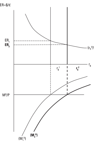
Figure 7-1: Increase in U.S. output.
Everything else constant, an increase in U.S. output or real income leads to an increase in the demand for money in the United States. As a result, the U.S. real interest rate increases.
Because of a higher real interest rate in the U.S. money market, you see an increase in the foreign exchange market in the perfectly inelastic curve that reflects the level of the real interest rate on the dollar-denominated security. This increase changes the equilibrium exchange rate from ER1 to ER2. Therefore, an increase in U.S. output with no change in the Eurozone leads to the appreciation of the dollar against the euro.
Increase in Eurozone’s output
Continue working with the dollar–euro exchange rate. This exercise indicates the change in output as well, but this time, everything else constant, you assume an increase in Eurozone’s output. Having an exercise with this assumption is important for the following reason: When you use the dollar-euro exchange rate, the explicit money market indicates the U.S. money market. Because the MBOP considers money markets of both the U.S. and the Eurozone, you may ask where the Eurozone’s money market is, or which curve indicates the Eurozone’s money market. This example is helpful in answering this question.
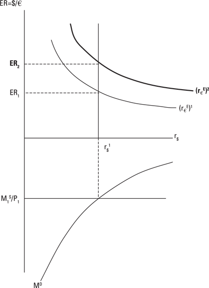
Figure 7-2: Increase in Eurozone’s output.
Remember, changes in any country’s output in this model result in changes in the demand for money. In Figure 7-2, the explicit money market is the U.S. money market; the Eurozone’s money market is reflected in the downward-sloping parity curve.
Also remember what the parity curve represents. In Figure 7-2, it implies the expected real return on the euro-denominated security in dollars. In other words, it shows:
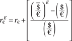
In this equation, r€ indicates the real interest rate in Euro-zone’s money market, determined by the money demand and supply curves. If it’s helpful for you, you can graph Euro-zone’s money market, as in Figure 7-3. This figure shows that, because output is held constant along the money demand curve, an increase in output increases the money demand curve, thereby increasing the real interest rate in Eurozone.

Figure 7-3: The effects of increase in Eurozone’s output on Eurozone’s money market.
Apply the increase in r€ in the money market to the previous parity equation. r€ in the equation increases, which increases the value of the parity curve. The parity curve in Figure 7-2 then also increases.
In this case, you predict that an increase in Eurozone’s output leads to the depreciation of the U.S. dollar.
Applying Nominal Shocks to MBOP
Unlike real shocks, such as a change in a country’s output, nominal shocks require you to conduct both short- and long-run analysis. Remember short-run refers to a period during which the value of a nominal variable is fixed or sticky. The long-run refers to a period during which all nominal variables change. (See Chapter 6 for discussions on the short- and long-run.)
The most important nominal variable in the MBOP is the nominal money supply. If a change in the nominal money supply occurs, the real money supply changes in the short run because of sticky prices. However, prices do not remain sticky in the long-run. They adjust in the direction proposed by the Quantity Theory of Money, and the money market goes back to its initial equilibrium.
As discussed in Chapter 6, the Quantity Theory of Money states that the percent change in the nominal money supply equals the percent change in the average price level in the same direction. For example, a 3 percent increase in the nominal money supply increases the average price level by 3 percent.
Suppose the central bank increases the nominal money supply. Assuming sticky prices (see Chapter 6), the real money supply increases in the short run. Because the Quantity Theory of Money implies that, in the long run, prices increase at the same rate as the increase in the nominal money supply, then as prices increase, the real money supply declines to its original level.
In the following, you analyze the short- and long-run effects of an increase in the nominal U.S. money supply on the dollar–euro exchange rate. This analysis is conducted first assuming no overshooting and then assuming overshooting. The term overshooting refers to a large, short-run change in the exchange rate (appreciation or depreciation) due to a nominal shock such as the change in the nominal money supply. Because overshooting indicates such a large increase or decrease in the exchange rate in the short-run, there will be some adjustments until the exchange rate settles at its long-run value.
You will see that the difference between the analysis with and without overshooting lies in the timing of changes in the expected exchange rate, which you hold constant until now. In the case of overshooting, you assume that investors adjust their expectations regarding the exchange rate in the short-run. If investors adjust their expectations regarding the exchange rate in the long-run, there will not be an overshooting.
Short- and long-run effects of a nominal shock — without overshooting
To start, I give you an example without overshooting because it’s an easier start. Figure 7-4 shows both the short- and long-run effects of an increase in the U.S. nominal money supply on the dollar–euro exchange rate without overshooting. In Figure 7-4, the initial real interest rate in the U.S. money market is r1$, and the initial dollar–euro exchange rate in the foreign exchange market is ER1.
When the central bank increases the U.S. nominal money supply, assuming sticky prices in the short run, an increase in the nominal money supply leads to an increase in the real money supply (MS2/P1). The resulting decline in the U.S. real interest rate (from r1$ to r2$) shifts the curve indicating the real return on the dollar-denominated security in the foreign exchange market to the left. As a result, in the short run, the dollar depreciates from ER1 to ERSR. Note that no change occurs in the parity curve; therefore, (rE€)1 is still the relevant parity curve in the short run.
In the long run, prices adjust according to the Quantity Theory of Money. In this case, the rate of increase in prices equals the rate of increase in the nominal money supply. Therefore, the long-run real money supply (MS2/P2) is the same as the initial real money supply (MS1/P1). In other words, the U.S. money market goes back to its initial equilibrium, where r1$ is the real interest rate.
Now you look at the foreign exchange market and determine where the long-run dollar–euro exchange rate is going to be. Consider the downward-sloping parity curve again. In Figure 7-4, the parity curve indicates the expected real return on the euro-denominated security in dollars.
In the next equation, r€ indicates the real interest rate on the euro-denominated security and is determined by the Eurozone’s money market. The term in brackets shows the expected change in the dollar–euro exchange rate. Therefore, the parity curve, or rE€, implies the expected real return on the euro-denominated security in dollars.


Figure 7-4: Exchange rate and increase in the nominal money supply (without over-shooting).
Now focus on the expected dollar–euro exchange rate, which refers to the expected future spot rate some time from now. The MBOP without overshooting allows investors to change their expectation regarding the future spot rate only in the long run, after the adjustments in the price level take place.
Therefore, when the money market goes back to its initial equilibrium in the long run, investors in the foreign exchange market make an upward adjustment in the expected dollar–euro exchange rate. An upward adjustment in the expected dollar–euro exchange rate is consistent with the expected depreciation of the dollar. This adjustment increases the value of the bracket in the parity equation, thereby shifting the parity curve up from (rE€)1 to (rE€)2.
The shift in the parity curve brings the foreign exchange market into equilibrium, which is now consistent with the money market equilibrium. Note that, in terms of the level of exchange rate, the short- and long-run exchange rates are the same. This is shown as ERSR=ERLR on Figure 7-4. However, while the short- and long-run exchange rates are the same, the long-run exchange rate is on the new parity curve, which is (rE€)2 on Figure 7-4.
In short, you predict depreciation in the dollar (or appreciation in the euro) when the U.S. nominal money supply increases.
Short- and long-run effects of a nominal shock — with overshooting
Figure 7-5 shows the short- and long-run effects of an increase in the U.S. nominal money supply on the dollar–euro exchange rate, now with overshooting. In Figure 7-5, the initial real interest rate in the U.S. money market and the initial dollar–euro exchange rate in the foreign exchange market still are r1$ and ER1.
The short-run analysis, assuming overshooting, starts just like the previous analysis without overshooting. Figure 7-5 indicates that following an increase in the U.S. nominal money supply, and assuming sticky prices in the short run, the real money supply increases from MS1/P1 to MS2/P1. Again, this change results in a lower real interest rate in the money market (r2$).
In the case of overshooting, investors adjust their expectations regarding the future spot rate upward, and the parity curve increases in the short run. This adjustment creates a larger short-run depreciation of the dollar. Note that the short-run exchange rate that is consistent with the short-run equilibrium real interest rate in the money market (r2$) is ERSR. In other words, the exchange rate overshoots to ERSR.
In the long run, prices adjust according to the Quantity Theory of Money. In the money market, the increase in prices is proportional to the increase in the initial nominal money supply. Therefore, the long-run real money supply (MS2/P2) is the same as the initial real money supply (MS1/P1). The U.S. money market goes back to its initial equilibrium, where r1$ is the real interest rate.
As the money market returns in the long run to its initial equilibrium, ERLR marks the equilibrium exchange rate. Note that the movement from ERSR to ERLR implies appreciation in the dollar; however, the dollar remains depreciated compared to the initial exchange rate ER1.

Figure 7-5: Exchange rate and increase in the nominal money supply (with over-shooting).
The concept of overshooting is one explanation for the surprisingly high volatility in exchange rates. Most short-term fluctuations in exchange rates don’t reflect changes in fundamentals, such as changes in monetary policy or output. The overshooting argument indicates that short-run changes in exchange rates can result from adjustments. For example, as Figure 7-5 shows, appreciation in the dollar from ERSR to ERLR is not related to a change in monetary policy; instead, it reflects the adjustment in the real money supply when prices adjust.
Comparing MBOP with and without overshooting
Because Figures 7-4 and 7-5 are drawn separately, you may not realize the following. The only difference overshooting introduces is the difference in short-run exchange rates. The short-run exchange rate with overshooting (ERSR in Figure 7-5) is higher than the short-run exchange rate without overshooting (ERSR in Figure 7-4). However, the long-run exchange rate (ERLR) is the same in both figures.
Figure 7-6 shows Figures 7-4 and 7-5 side by side, to show that overshooting matters only in the short run. The model with overshooting implies a larger short-run response of investors to changes in monetary policy, indicated by the upward shift of the parity curve in the short run. In the model without overshooting, however, investors adjust their expected exchange rate when prices change in the long run.
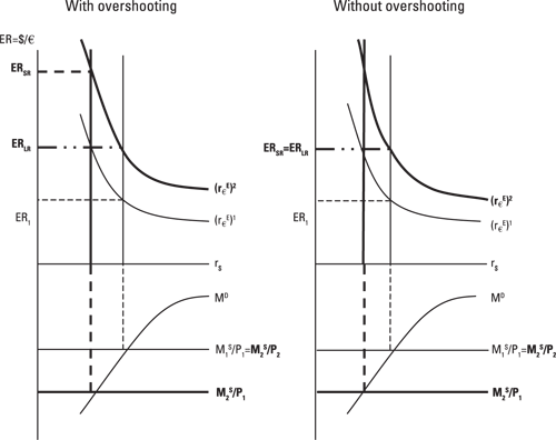
Figure 7-6: Exchange rate and increase in the nominal money supply (with and without over-shooting).
In terms of the long run, Figure 7-6 indicates that, with or without overshooting, the long-run exchange rate settles at the long-run exchange rate of ERLR. Note that, in both models, the ERLR is on a higher parity curve, indicated by (rE€)2.
Keeping It Straight: What Happens When We Use a Different Exchange Rate?
This section introduces exercises with a different exchange rate. As discussed earlier, that the variables associated with the money and foreign exchange markets of the MBOP must be consistent with each other. Using a different exchange rate motivates you to consider the setup of the MBOP once again.
Additionally, the example for the nominal shock implies not only a different exchange rate, but also a different change in the nominal money supply than in the previous example.
Effects of a real shock
In this example, the real shock is a decline in U.S. output. You use the euro–dollar exchange rate.
Figure 7-7 indicates the exchange rate in the foreign exchange market as the euro–dollar exchange rate. Because the exchange rate is expressed as the number of euros per dollar (in other words, in euros), the x-axis of the foreign exchange model must be in euros as well, to indicate the real return on the euro-denominated security. Then the parity curve in the foreign exchange market shows the expected real return on the dollar-denominated security in euros, or r$E.
In terms of the money market, the x-axis of the foreign exchange market becomes the y-axis of the money market. Therefore, the demand for and supply of money in Figure 7-7 are the Eurozone’s.
The initial equilibrium in the foreign exchange is ER1; it’s r€1 in the money market. Because the shock is a decline in U.S. output, you first want to identify what is affected by a change in U.S. output. Remember that a country’s output is a ceteris paribus condition along the money demand curve. But the demand for money in the figure is the demand for euros in Eurozone, so it does not change when U.S. output changes. The demand for money in the Eurozone changes when Eurozone output changes. Because in this example the U.S. output changes and this change affects the U.S. money market, you need to locate where the U.S. money market is. In Figure 7-7, the U.S. money market is captured along the parity curve in the foreign exchange market.
In Figure 7-7, the parity curve implies:
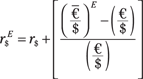
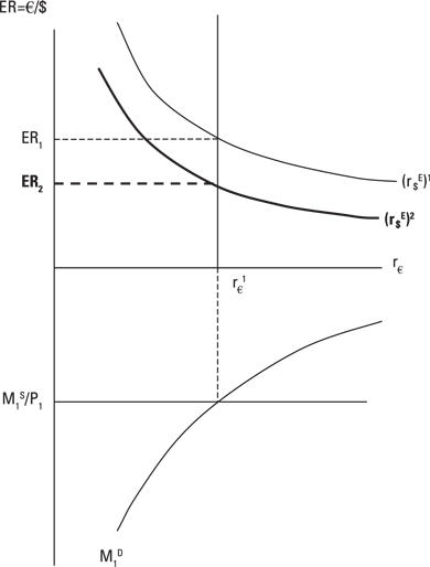
Figure 7-7: Decline in U.S. output.
This parity curve indicates the expected real return on the dollar-denominated security in euros. The U.S. real interest rate (r$) that’s determined in the U.S. money market is part of the parity curve. A decline in U.S. output decreases the money demand, thereby decreasing the U.S. real interest rate, which then decreases the value of this equation and shifts the parity curve down in Figure 7-7.
Based on this analysis, you predict the appreciation of the euro (or depreciation of the dollar).
Effects of a nominal shock
This nominal shock comes straight from the headlines. On October 7, 2009, The Wall Street Journal reported that the Australian Central Bank had raised its key interest rate (“Australia Rate Rise Poses a Global Policy Challenge,” Section A14).
Note that the article mentions the key interest rate, not the nominal money supply. You can interpret the increase in the key interest rate as equivalent to a decline in Australia’s nominal money supply (see Chapter 6).
Figures 7-8 and 7-9 show the effects of this monetary policy change without and with overshooting, respectively. In this example, you want to see the results of the changes in Australia’s monetary policy explicitly in the Australian money market. Therefore, the explicit money market is the Australian money market, and the y-axis of the money market indicates the Australian real interest rate. In the foreign exchange market, the y-axis of the money market becomes the x-axis of the foreign exchange market. Because it is in Australian dollars, the exchange rate is in Australian dollars as well. This fact explains why you work with the Australian dollar–U.S. dollar exchange rate in this model.
Exchange rate without overshooting
Start with Figure 7-8, which shows the change in the exchange rate without overshooting. In the short run, a decline in the nominal quantity of money leads to a decline in the real quantity of money, assuming sticky prices. This increases the Australian real interest rate. In the foreign exchange market, you also observe a higher real interest rate, which is consistent with an exchange rate that’s lower than the initial exchange rate ER1. ERSR indicates the short-run exchange rate, which implies an appreciation of the Australian dollar in the short run.
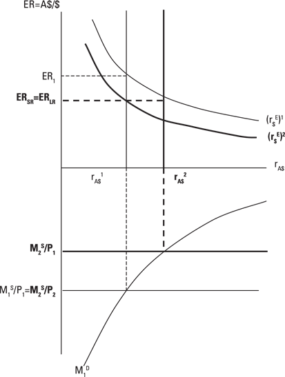
Figure 7-8: Short- and long-run effects of Australia’s contractionary monetary policy (without overshooting).
 This term contractionary is generally used with respect to monetary policy, where a contractionary monetary policy refers to a decline in money supply and/or an increase in a central bank’s key interest rate. This particular monetary policy makes money scarce, thereby increasing its price, which is the interest rate. In contrast, expansionary monetary policy indicates an increase in money supply and/or a decline in a central bank’s key interest rate, which makes money relatively more abundant, thereby decreasing its price (or the interest rate).
In the long run, prices adjust downward at the same rate as the decline in the nominal money supply. Therefore, the money market returns its initial equilibrium, where the real interest rate is rA$1. As the money market returns to its initial equilibrium, investors in the foreign exchange market make a downward adjustment in their expected exchange rate. Consider the parity curve that implies the expected real returns on a dollar-denominated security in Australian dollars:
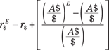
A downward adjustment in the expected Australian dollar–U.S. dollar exchange rate implies an expected appreciation in the Australian dollar. This appreciation decreases the parity curve. Although the long-run exchange rate (ERLR) is the same as the short-run exchange rate, the former is associated with a lower parity curve. And the long-run current exchange rate implies an appreciation of the Australian dollar (or depreciation of the U.S. dollar).
Exchange rate with overshooting
In Figure 7-9, you see the change in the exchange rate with overshooting. As discussed earlier, overshooting happens in the short run. Again, the Australian central bank decreases the nominal money supply and, assuming sticky prices, the real money supply declines. This leads to a higher real interest rate, rA$2, in the Australian money market. Now investors in the foreign exchange market make a downward adjustment in their expected exchange rate in the short run, implying an expected appreciation in the Australian dollar. Therefore, the parity curve declines in the short run, causing an overshooting in the exchange rate to ERSR.
As prices adjust downward in the long run, the real money supply goes back to its original position, bringing the real interest rate down to rA$1. The real interest rate declines in the money market; in the foreign exchange market, the exchange rate increases to ERLR. Although the change from ERSR to ERLR implies depreciation in the Australian dollar after an initial appreciation, ERLR indicates that the net result is an appreciation in the Australian dollar compared to the initial exchange rate, ER1.
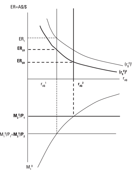
Figure 7-9: Short- and long-run effects of Australia’s contractionary monetary policy (with overshooting).
Comparing Predictions of MBOP and the Demand–Supply Model
In economics, alternative theories seek to explain the determination of the same variable. And alternative theories apply to exchange rate determination as well. In Chapter 5, you predict the changes in the exchange rate according to the demand–supply model. In Chapters 6 and 7, the MBOP explains the changes in the exchange rate.
When you compare alternative theories, be aware of the differences in their approach to the subject:
![]() The demand–supply model considers both trade and portfolio flows. The MBOP considers only the portfolio flows and views the exchange rate determination exclusively from the viewpoint of international investors.
The demand–supply model considers both trade and portfolio flows. The MBOP considers only the portfolio flows and views the exchange rate determination exclusively from the viewpoint of international investors.
![]() As opposed to the MBOP, the demand–supply model does not explicitly deal with monetary policy; instead, it deals with its consequences, which imply the changes in the price level. The relevant shock in the demand–supply model is the changes in the inflation rate; the MBOP uses the changes in the nominal money supply as a nominal shock to the money market.
As opposed to the MBOP, the demand–supply model does not explicitly deal with monetary policy; instead, it deals with its consequences, which imply the changes in the price level. The relevant shock in the demand–supply model is the changes in the inflation rate; the MBOP uses the changes in the nominal money supply as a nominal shock to the money market.
![]() Contrary to the MBOP, the demand–supply model does not explicitly refer to the short- and long-run analysis. However, throughout this chapter you read that a change in the nominal money supply will lead to a change in prices in the long-run. The fact that the change in the inflation rate is a shock in the demand–supply model indicates that this model implicitly considers the long run.
Contrary to the MBOP, the demand–supply model does not explicitly refer to the short- and long-run analysis. However, throughout this chapter you read that a change in the nominal money supply will lead to a change in prices in the long-run. The fact that the change in the inflation rate is a shock in the demand–supply model indicates that this model implicitly considers the long run.
Despite differences in their approach to exchange rate determination, both theories generally provide the same prediction on the effects of similar shocks to the exchange rate.
In terms of the effects of changes in real interest rates, both theories offer the same prediction. First, the higher real interest country’s currency is expected to appreciate. For example, Figure 5-8 in Chapter 5 shows that an increase in Eurozone’s real interest rate leads to an appreciation in the euro against the dollar. You see the same result in this chapter in Figures 7-8 and 7-9. However, as indicated previously, the difference is that the demand–supply model doesn’t indicate the source of the change in the real interest rate (it can be related to money supply or money demand). The MBOP, on the other hand, considers a shock to money supply or demand, which changes the real interest rate in the money market.
Second, both theories predict depreciation in the higher inflation country’s currency. Again, these theories use different approaches when determining the effects of inflation on the exchange rate. Whereas the demand–supply model uses a trade-related explanation, the MBOP relates the change in the inflation rate to the change in the nominal money supply. In the MBOP, changes in the money supply lead to changes in the price level as proposed by the Quantity Theory of Money. Despite different theoretical framework, Figure 5-6 in Chapter 5 indicates that a higher U.S. inflation rate leads to depreciation of the U.S. dollar. Figures 7-4 and 7-5 predict the same result.
Empirical evidence verifies the predictions of both models with respect to the real interest rate and the inflation rate.
The only difference in these theories’ predictions occurs in terms of the changes in output. Output is a trade-related factor in the demand–supply model. In this model, a higher output motivates a country’s citizens to buy more foreign goods (at the given exchange rate). In Figure 5-7 in Chapter 5, you see that a higher output growth in the Eurozone leads to depreciation of the euro. In the MBOP, output is related to the money demand and affects the real interest rate. Higher output increases the money demand and, thereby, the real interest rate. Figures 7-2 and 7-4 indicate appreciation of the higher output country’s currency. The predictions of these two theories regarding output are conflicting, and empirical evidence can help show which is correct. In this case, empirical evidence supports the predictions of the MBOP.
To conclude the theory part, the demand-supply model provides a simple model of the exchange rate determination. While the MBOP is more complex, it is a modern approach to exchange rate determination.