Chapter 6

Setting Up the Monetary Approach to Balance of Payments

In This Chapter

Examining the foreign exchange market from an international investor’s point of view

Relating the domestic money markets of two countries to the foreign exchange market

Explaining how investors interpret the changes in monetary policy

Explaining how investors’ interpretation of monetary policy affects exchange rates

Chapter 5 covers the demand-supply approach to exchange rate determination. This chapter introduces an alternative theory of exchange rate determination. While the demand-supply model assumes that both international trade- and international investment-related factors change exchange rates, the Monetary Approach to Balance of Payment (MBOP) takes only international investment into account. In other words, the MBOP views the subject of exchange rate determination from the point of view of international investors.

In this chapter, you’ll imagine investors trying to decide between two securities denominated in two different currencies. The answer to the question “How will they decide?” lies in the center of the MBOP’s method of exchange rate determination. As investors favor one country’s security over the other country’s security, their decision affects the exchange of currencies and therefore leads to appreciation or depreciation of currencies.

You may be asking what the name Monetary Approach to Balance of Payment suggests. Here I break it down into two parts:

Monetary: The term Monetary in the name of this particular approach to exchange rate determination reveals interesting insights regarding the decision-making process of international investors. It means that investors keep an eye on the interest rates in the money markets of two countries. Additionally, because changes in monetary policies of these countries change their interest rates, investors pay attention to changes in monetary policies of these countries as well.

Balance of Payments: The Balance of Payments (BOP) indicates an account that keeps track of a country’s transactions with other countries. The BOP captures trade in goods and services as well as the flow of funds (investment, loans, and so on) between the home country and the rest of the world. Historically, the Monetary Approach to Balance of Payments indicated the theory that explains the effects of the changes in a country’s money market on its BOP or its transactions with the rest of the world. Then, the same name was used for the effects of the changes in the money market on exchange rates.

Combining these two points, you may view the name of the theory presented in this chapter (the Monetary Approach to Balance of Payments) as the Monetary Approach to Exchange Rate Determination.

Discovering the MBOP’s Approach to Exchange Rates

This section provides a discussion regarding the assumptions and the general setup of the MBOP. It also compares the MBOP’s approach to the demand–supply model (for more on the demand–supply model, see Chapter 5). In Economics, alternative theories explain the determination of a relevant variable. Looking at the approach of competing theories to a variable such as the exchange rate, you can see how and why each theory provides a certain prediction. Comparing the predictions of different theories and identifying the common factors in the determination of a variable, such as the exchange rate, is important for the empirical verification of these theories.

Viewing the basic assumptions

As in the case of the demand-supply model (see Chapter 5), the MBOP has its own assumptions:

No government intervention: The MBOP assumes flexible exchange rates. In other words, the currencies in question are traded in foreign exchange markets with minimal or no government intervention.

The MBOP also provides insights into the credibility of currency pegs and the possibility of a currency crisis. Chapter 13 makes references to the MBOP in this context.

International investor behavior: The most important characteristic of the MBOP is its exclusive focus on the behavior of international investors. The MBOP considers an international investor who is trying to decide between securities denominated in two different currencies. Therefore, it is not surprising that the MBOP is also called the Asset Approach to Exchange Rate Determination.

Changes in real returns: The term monetary in the MBOP emphasizes the relevance of the changes in monetary policy and the resulting changes in real returns on securities denominated in different currencies. After investors observe these changes in real returns, they express their preference for a security, which leads to buying or selling certain currencies and, therefore, changes in the exchange rate.

Setting the MBOP apart

When comparing the assumptions of the MBOP to those of the demand–supply model (see Chapter 5), you notice that the MBOP focuses exclusively on investors’ decisions between two securities. The MBOP considers investment-related factors in exchange rate determination compared to the demand-supply model, which considers both investment- and trade-related factors. Since the interest rate is an international investment-related factor, both theories use this factor in explaining the changes in exchange rates.

In fact, investors in both theories compare the real interest rates in two countries. The difference between these theories regarding real interest rates lies whether the source of the change in the real interest rate is explicitly discussed. The demand–supply model doesn’t explicitly consider the source of the change in interest rates. It just assumes that the real interest rate in a country changes. However, as the beginning of this chapter notes, the MBOP relates the changes in the money markets of countries to the changes in exchange rates. Because money markets determine the real interest rates of countries in the MBOP, this theory explicitly shows how the changes in the market markets of both countries affect these countries’ real interest rates and subsequently the exchange rate.

Therefore, in later sections of this chapter, you see that the MBOP consists of the combination of two models: the money market and the foreign exchange market. Basically, the changes in the money market lead to changes in real returns on securities denominated in different currencies. Then investors’ subsequent reaction to the changes in real returns leads to changes in the relevant exchange rate. Therefore, this chapter develops the MBOP in three stages: the money market, the foreign exchange market, and the combination of the money and foreign exchange markets or the combined MBOP.

Explaining the Money Market

You may think of money market as a familiar term. A word of caution: sometimes the same term has a different content in Finance than in Economics. Money market is one of these terms. In Finance, the term money market is used to refer to securities whose maturity is one year or less (such as Treasury bills, commercial paper, and so on). In Economics, money market or orange market has essentially the same meaning. A market has a demand and a supply curve that shows the demand for and supply of the good in question.

As discussed in Chapter 5, when the market in question is the orange market, this market is illustrated by putting the quantity of oranges on the x-axis and the price of oranges on the y-axis. In this case, the curves of the model indicate the demand for and the supply of oranges. You consider the money market in the same way. The quantity of money goes to the x-axis and the price of money, which is the real interest rate, goes to the y-axis. The money demand represents people’s liquidity preference. The money supply indicates the bills and coins issued by the country’s central bank and various kinds of deposits held by public at depository institutions such as banks, credit unions, and so on. When the money demand and money supply are determined, an equilibrium real interest rate is reached in the money market.

This section also discusses the major sources of changes in the real interest rate. Identifying these changes in the real interest rate is important because later in this chapter you connect these changes in the money market to the changes in the exchange rate.

Demand for money

The demand curve for money is called the liquidity preference, for a good reason. This curve drawn in the real interest rate/real quantity of money space shows how much money you want to keep in your pocket or in a non-interest-earning account, such as your debit account. Of course, a good reason to keep money with you (or on your debit account) is the relevance of money as the medium of exchange. Every time you want to have pizza, you don’t want to liquidate some of your assets, for example government bonds!

A standard money demand example

Figure 6-1 indicates the x-axis as the real quantity of money, where the nominal quantity of money (M) is divided by the average price level (P). For example, if you have $100 and tall lattes of $2 each are the only good you consume, your real money, or the purchasing power of your nominal money, equals 50 lattes ($100 ÷ $2).

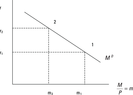
Figure 6-1: The money demand curve.

In Figure 6-1, the y-axis refers to the real interest rate (the nominal interest rate minus the inflation rate). You see that the money demand curve is a downward-sloping curve in the real interest rate-real money space. When the real interest rate increases (moving from Point 1 to Point 2 in Figure 6-1), the quantity of real money demanded declines. In other words, people carry less money to take advantage of higher real interest rates. Similarly, when the real interest rate is lower (moving from Point 2 to Point 1 in Figure 6-1), the quantity of real money demanded is higher because people are losing a smaller amount of interest income by keeping more money.

Drawing the money demand curve in the real interest rate-real quantity of money space is one of the alternative explanations of the money demand, which is commonly used in the MBOP. The money demand can also be derived in the nominal interest rate-nominal quantity of money space.

An example for the shift in the money demand

What would shift the money demand curve? To shift the money demand curve, or any curve in economics, you need to assume a change in the value of a ceteris paribus condition associated with this curve. Ceteris paribus translates to “all other things being equal or held constant.” In other words, the assumption is that the values of certain variables are assumed to be constant along the money demand curve, no matter where you are on the curve, Point 1 or Point 2 on Figure 6-1.

In the case of the money demand curve, one ceteris paribus condition is worth mentioning: real income, which can be measured as real GDP or real income or output of a country (Y).

Figure 6-2 provides an example for a shift in the money demand curve. The shock associated with this shift is an increase in output. As output or real income increases, at the given real interest rate, the quantity of real money demanded increases as well. Because the value of the X variable increases at the given level of the Y variable, you refer to this shift as an increase in the money demand curve. Similarly, if a decline in the output of a country takes place, you decrease the money demand curve, which leads to a lower real quantity of money demanded at the given real interest rate.

Figure 6-2: A shift in the money demand curve.

Supply of money

In the money market of the MBOP, the central bank controls the nominal money supply (MS). Given the average price level, the nominal money supply (MS) divided by the average price level (P) defines the real money supply (mS). Figure 6-3 shows the real money supply as a perfectly inelastic curve. Additionally, the central bank controls the nominal money supply. Therefore, the nominal money supply is one of the ceteris paribus conditions along the real money supply curve.

A perfectly inelastic (vertical) curve in Figure 6-3 indicates that the curve has an x-intercept. In other words, the curve is associated with a given level of the x- variable, in this case, the real quantity of money. A perfectly inelastic curve such as the real money supply curve in Figure 6-3 also indicates that the real quantity of money (m1) does not vary with the real interest rate (r). The real interest rate can be higher or lower; the x-intercept or m1 remains the same. In contrast, a perfectly elastic (horizontal) curve has a y-intercept. This time, there is a level of the real interest rate that doesn’t respond to changes in the quantity of real money (m) on the x-axis.

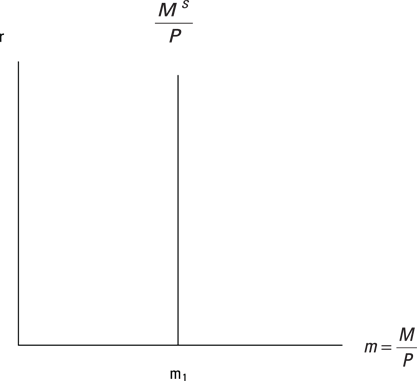
Figure 6-3: The real money supply.

The perfectly inelastic (vertical) real money supply curve in Figure 6-3 may seem surprising. This particular real money supply curve implies that the central bank focuses on the quantity of money as the monetary policy tool. In recent decades, most central banks use a key interest rate (such as the Fed’s Federal Funds Rate) instead of the quantity of money when conducting monetary policy. However, for our purpose it does not matter whether the real money supply curve is perfectly inelastic (the central bank’s policy tool is the quantity of money) or perfectly elastic at the given interest rate (the central bank’s policy tool is a key interest rate).

Another ceteris paribus condition along the real money supply curve is the average price level in a country. Changes in the nominal money supply lead to changes in the price level. The question is, when? To help answer that question, think about the predictions of two major schools of thought in economics (they coincide with the long-run and short-run analysis in economics):

The classical–neoclassical school: This school relies on the Quantity Theory of Money. This theory predicts that the changes in the price level equal the changes in the nominal money supply. In this case, a positive relationship exists between the changes in the nominal money supply and the price level. Therefore, if a central bank increases the nominal money supply by 5 percent, it creates 5 percent inflation.

The classical-neoclassical school relies on the long-run view. In economics, the long-run represents the run, during which all nominal variables adjust. Figure 6-4 illustrates the situation in which the nominal money supply has increased from M1 to M2. According to the long-run view, the average price level increases at the same rate from P1 to P2, leaving the real money supply unchanged (m1).

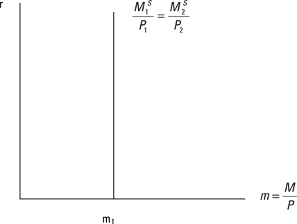
Figure 6-4: An example of the increase in the nominal money supply (classical–neoclassical school; long-run view).

The Keynesian school: You may have heard about Keynes’s famous phrase: “In the long run, we are all dead.” Clearly, Keynes did not care much about the long-run analysis that assumes that all nominal variables adjust. Instead, he introduced the notion of the short run, during which a nominal variable remains sticky. A sticky nominal variable is a variable that does not change, per definition, during the short-run. The MBOP assumes that prices of goods and services in an economy are sticky.

Various explanations seek to tell why prices are sticky. These explanations can be summarized as menu cost. Basically, menu costs imply the assumption that frequently changing prices of goods and services are annoying to consumers. Therefore, firms may not change the prices of their products every time their production costs change. They may wait until the current price is no longer sustainable at their new cost structure. However, note that when firms adjust their prices (upward or downward), the average price level remains sticky at a new level.

Assuming sticky prices, if a central bank increases the nominal money supply, the real money supply increases. Figure 6-5 shows this result. The initial nominal money supply, M1, increases to M2. Because prices are sticky in the short run, the initial price level, P1, remains the same after the increase in the nominal money supply. Because you are dividing a larger number (M2) by the same price level (P1), there is an increase in the real money supply curve.

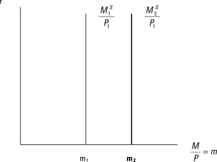
Figure 6-5: An example of the increase in the nominal money supply (Keynesian school; short-run view).

Similarly, if there is a decline in the nominal money supply, assuming sticky prices, this time the real money supply declines, decreasing the real money supply curve.

In the next section, both the short- and long-run analyses are applied when there is a change in the nominal money supply.

Money market equilibrium

When the money demand and supply curves are put together, you can view the money market. Figure 6-6 indicates the money market equilibrium, with the equilibrium real interest rate, r1, and the equilibrium quantity of real money, m1.

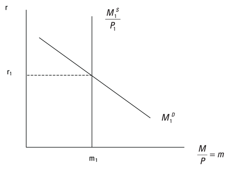
Figure 6-6: The money ­market.

Remember the variables that can shift the money demand and supply curves. In the next example, a change in the country’s output and nominal money supply is applied to the money market. You can predict how the real interest rate and the real quantity of money in the money market change.

We start with an increase in output. Figure 6-7 shows that an increase in output increases the money demand curve, which, in turn, increases the real interest rate without changing the quantity of real money.

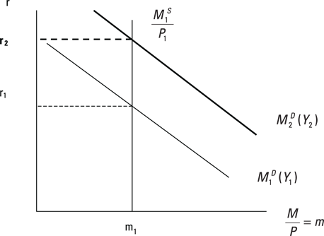
Figure 6-7: Effects of an increase in output.

Now assume an increase in the nominal money supply, shown in Figure 6-8. Because there is a change in a nominal variable this time, the short- and long-run predictions differ.

Figure 6-8: Short- and long-run effects of an increase in the nominal money ­supply.

In the short run, you assume sticky prices. At the same prices, if the initial nominal money supply of M1 increases to M2, the real money supply also increases. As a result, the real money supply curve increases (shifts to the right). Therefore, in the short run, you predict a lower real interest rate (r2) and a higher quantity of real money (m2).

To express your long-run predictions, make use of the Quantity Theory of Money. This theory states that, in the long run, the price level increases at the same rate at which the nominal money supply increased. Therefore, you expect the percent increase from P1 to P2 to match the increase in the nominal money supply from M1 to M2. In this case, the real money supply curve returns to its original position, indicating r1 as the equilibrium real interest rate and m1 as the equilibrium real quantity of money. The real quantity of money is the same as before m1 because the price level and the nominal money supply have increased by the same proportion (M1/P1 = M2/P2).

Taking On the Foreign Exchange Market

Now the focus is on the foreign exchange market. The most important insight that you want to get from the foreign exchange market is the determination of the exchange rate. As discussed previously in this chapter, the approach to and the assumptions associated with exchange rate determination are the key to illustrating the foreign exchange market. Remember that the exchange rate determination based on the MBOP adopts an asset approach, which is based on the behavior of international investors contemplating investing in securities of different denominations.

Think of it this way: You are an American investor trying to choose between a dollar- and euro-denominated security of comparable risk and maturity. Suppose you observe that the annual real rate of return on comparable dollar- and euro-denominated securities is 5 percent and 6 percent, respectively. Are you thinking about picking the euro-denominated security? Hopefully not! You don’t want to compare the real returns on securities that are denominated in different currencies; it’s like comparing apples and oranges.

Therefore, this section first expresses the real returns on securities denominated in different currencies in a comparable format. After this discussion, grasping the meaning of the curves in the foreign exchange market is easier.

Asset approach to exchange rate ­determination

This section provides how-to information on comparing the real returns on dollar-denominated securities with the real returns on euro-denominated securities. The concept that makes this comparison possible is the expected change in the exchange rate.

For example, when you invest in a euro-denominated security, you hope to make money in two ways. First, you expect to earn a return on this security you are planning to hold. Suppose that r€ is the real return on euro-denominated securities.

Second, you, the American investor, convert your dollars into euros, buy euro-denominated securities, earn returns in euros, and convert your euro earnings into dollars. Therefore, you care about the future exchange rate that you observe when you convert your earnings in euros into dollars. However, you are investing in euro-denominated securities now, and you don’t know for sure what the dollar–euro exchange rate is going to be in the future — say, a year from now. Still, you need to have an expected dollar–euro exchange rate in mind.

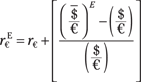
Clearly, you can observe the current exchange rate. We can call the current time t. Suppose you have an expectation of what the dollar–euro exchange rate is going to be at a future date. You use the current and expected exchange rate to calculate the expected percent change in the exchange rate using the following formula:

where:

ER = Exchange rate

Note the line over the expected exchange rate, which indicates that you are holding its value constant. Later in this chapter, but especially in the next chapter (Chapter 7), you change this assumption.

Now you, the investor, can make the appropriate comparison between the real return on a risk- and maturity-comparable dollar- and euro-denominated security. You are indifferent between these securities if the following parity condition holds:

Note that the previous formula drops the time subscript for simplicity.

where:

r$ = Real return on the dollar-denominated security (in dollars)

r€ = Real return on the euro-denominated security (in euros)

The right side of the equation expresses the expected real returns on the euro-denominated security in dollars. By adding the expected change in the exchange rate to the real return on the euro-denominated security, you account for two possible sources of your return from a euro-denominated security: the interest rate on the euro-denominated security (r€) and whether you will enjoy additional returns when you convert your earnings in euros into dollars. Now you can compare your earnings on a dollar-denominated security to your earnings on the euro-denominated security. In other words, you can compare the number of dollars you will have in the future from holding the dollar-denominated security to the number of dollars you will have in the future from holding the euro-denominated security.

Another way of expressing the parity condition is that the difference between the real return on a dollar-denominated security and that of a euro-denominated security in dollars must be zero:

Figure 6-9 shows four numerical examples to which you can apply the parity condition and decide which security gives you a higher real return. The second and third columns indicate the real return on the dollar- and euro-denominated securities, respectively. The fourth column shows the expected change in the exchange rate. The last column indicates the parity condition as the difference among these three variables, and the difference is zero. In other words, after adjusting for the expected changes in the exchange rate, a security denominated in euros offers the same (expected) real rate of return as the dollar-denominated security.

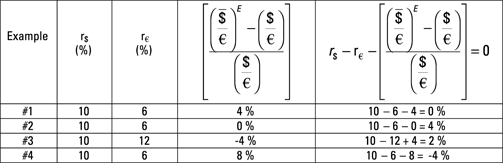
Figure 6-9: Interest parity example.

For simplicity, the real returns on the dollar-denominated security don’t change in Figure 6-9. However, you can see changes in the real returns on the euro-denominated security and the expected change in the exchange rate.

Take a look at Figure 6-9 and consider each example:

Example #1: The real return on the dollar- and euro-denominated security is 10 percent and 6 percent, respectively. Additionally, the expected change in the exchange rate indicates 4 percent depreciation in the dollar. In other words, if you invest in the euro-denominated security, in addition to earning 6 percent interest on the security, you earn 4 percent by holding a security whose currency is expected to appreciate. In this case, you earn 10 percent real return in either security. Therefore, you are indifferent between the dollar- and euro-denominated securities.

Example #2: The second example has the same real returns on the dollar- and euro-denominated securities, which are 10 percent and 6 percent, respectively. However, in this case, the expected exchange rate is the same as the current exchange rate, so the expected change in the exchange rate is zero. Now the real return on the dollar-denominated security exceeds that on the euro-denominated security by 4 percent. In this case, you want to invest in the dollar-denominated security.

Example #3: This example indicates the real returns on the dollar- and euro-denominated securities as 10 percent and 12 percent, respectively. However, the expected change in the exchange rate is –4 percent, which indicates a 4 percent appreciation in the dollar. This reduces your real return on the euro-denominated security in dollars to 8 percent, which is lower than the real return on the dollar-denominated security. In this case, you want to invest in the dollar-denominated security.

Example #4: The last example indicates that the real return on the dollar- and euro-denominated securities is 10 percent and 6 percent, respectively. The expected change in the exchange rate is 8 percent, which indicates a depreciation of the dollar by 8 percent. This means that your expected real return on the euro-denominated security is 4 percent greater than that on the dollar-denominated security. In this case, you want to invest in the euro-denominated security.

The next section derives the parity curve based on the discussion of the parity condition in this section, which is one of the curves in the foreign exchange market based on the MBOP.

The expected real returns curve

The aim is to develop the foreign exchange market. It means that there should be some curves describing the foreign exchange market. The discussion about the interest parity in the previous section provides a verbal description of one of the curves in the foreign exchange market. In this section, I show the transformation of explanations regarding the interest parity into a curve, called the expected real returns curve or the parity curve.

The foreign exchange market has the dollar–euro exchange rate on the y-axis and the real returns in dollars on the x-axis. Figure 6-10 illustrates the ­downward-sloping parity curve, which implies the expected real return on the euro-denominated security.

In all economic models, it’s important to be mindful of which market is considered. This consideration is also important in the MBOP. Additionally, because this model deals with an exchange rate and two countries’ real interest rates, you need to use the exchange rate and the real interest rates in a consistent manner. For example, in Figure 6-10, the foreign exchange market is in dollars. How do you know? Because the exchange rate on the y-axis implies the amount of dollars per euro, which is clearly in dollars. Also, if the exchange rate is in dollars, the x-axis has to indicate the real return in dollars, which can be the real return on the dollar-denominated security or the real return on the euro-denominated security in dollars. (There is another exercise at the end of this chapter, which helps you to keep the exchange rate and the real interest rates straight.)

Figure 6-10: Parity curve in the foreign exchange market.

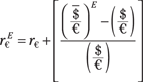
Now you know which variables are on the x- and y-axes of the model in Figure 6-10: the dollar-euro exchange rate and the real returns in dollars are on the y- and x-axis, respectively. But, remember from the discussion of the interest parity, you also need the information about the real returns on the euro-denominated security as well as its conversion into dollars. Therefore, the parity curve in Figure 6-10 indicates the right side of the parity equation:

Note that there is now an expectation superscript associated with the real returns on the euro-denominated security in dollars to emphasize the following idea. If you, an American investor, invest in dollar-denominated securities, you don’t need to deal with the expected exchange rate. However, if you want to consider a euro-denominated security, its return has to be comparable to that of the dollar-denominated security. In this case, you need to consider the expected exchange rate, because the current exchange rate is likely to change while you are holding the euro-denominated security. This is why it is appropriate to explain this parity curve as the expected real returns on euro-denominated security in dollars.

Based on the parity equation, the expected real return on the euro-denominated security in dollars is equal to the addition of the real return on the euro-­denominated security and the expected change in the exchange rate. At this point, it’s important to recognize that the real return on the euro-denominated security is determined in the Euro-zone’s money market, based on the discussion about the money market in the previous section. And the term in the bracket implies the expected change in the exchange rate, as you perceive it.

In Figure 6-10, it seems that a higher expected real return on the euro-­denominated security in dollars is associated with a lower dollar–euro exchange rate. Similarly, a lower expected real return on the euro-denominated security in dollars is associated with a higher dollar–euro exchange rate. This means that the dollar appreciates from Point 1 to Point 2 in Figure 6-10. Why is the parity curve downward-sloping in the exchange rate-real return space?

The answer lies in the parity condition. Continue assuming real returns on the dollar- and euro-denominated security; also assume that the expected exchange rate does not change. Note that the current exchange rate [($/€)t] is on the y-axis of the foreign exchange market. Because the aim here is to predict what the current exchange rate will be, it should be allowed to change. Also note that the same current exchange rate is used in the expected change in the exchange rate:

If the expected exchange rate is assumed to be fixed and the current exchange rate can change, you can show that depreciation of a country’s currency today lowers the expected real returns on the foreign security in domestic currency. Similarly, appreciation of the domestic currency today raises the returns on foreign currency deposits in domestic currency. Following are some numerical examples.

Suppose that the current dollar–euro exchange rate is $1.00 per euro, and the expected exchange rate next year is $1.05 per euro. Then the expected rate of depreciation in dollars is 5 percent ([1.05 – 1.00]/1.00 = 0.05, or 5 percent). This means that when you invest in a euro-denominated security, in addition to earning a return on this security, you receive an additional 5 percent return when you convert your euro earnings into dollars in the future.

Now suppose that current exchange rate suddenly depreciates to $1.03 per euro, but the expected exchange rate is still $1.05 per euro. You earn the same real return on the euro-denominated security. But what happens to your extra income that comes from the depreciation of the dollar? It’s smaller now because the expected depreciation of the dollar declines from 5 percent to 1.9 percent ([1.05 – 1.03]/1.03 = 0.019, or 1.9 percent). Because the real return on the euro-denominated security, or r€, has not changed, the expected real return on the euro-denominated security in dollars declines as the current dollar–euro exchange rate increases or the dollar depreciates (which is a movement from Point 2 to Point 1 in Figure 6-10).

Therefore, when holding the expected exchange rate constant, a negative relationship exists between the current dollar–euro exchange rate and the real returns on the euro-denominated security in dollars.

The other real returns curve

Remember you are trying to construct a graphical representation of the foreign exchange market. The current exchange rate is on the y-axis. The real returns in dollars are on the x-axis. And the last section added the downward-sloping parity curve (the expected real returns on euro-denominated security in dollar curve). When you inspect Figure 6-10, you see that so far there is one curve in the foreign market and there is yet no equilibrium exchange rate. The reason is that you could be anywhere on the parity curve, at Point 1 or Point 2, but you don’t know for sure. Therefore, you need another curve to complete the foreign exchange market.

At this point, it’s helpful to consider the parity condition again:

Looking at the parity condition again makes you realize that the discussion until now focused on the right side of the parity equation, which is shown in Figure 6-10 as the parity curve. Therefore, all you know by now is the expected real return on the euro-denominated security in dollars. But how can you compare the euro-denominated security to the dollar-denominated security, if you don’t know about the real return on the dollar-denominated security? The discussion needs to focus on the left side of the above parity equation.

As in the case of the euro-denominated security, the real return on the dollar-denominated security, r$, is determined in the U.S. money market based on the money demand and supply. Figure 6-11 illustrates the real return on the dollar-denominated security as a perfectly inelastic curve because the value of this variable is determined in the U.S. money market. Therefore, the real return on the dollar-denominated security doesn’t vary with the exchange rate.

Figure 6-11: Real return on the dollar-denominated security.

Of course, changes in the money market shift this curve. Figure 6-12 shows the effects of these changes in the money market on the foreign exchange market. Remember the variables that shift the curves in the money market, and try to explain the shifts in Figure 6-12.

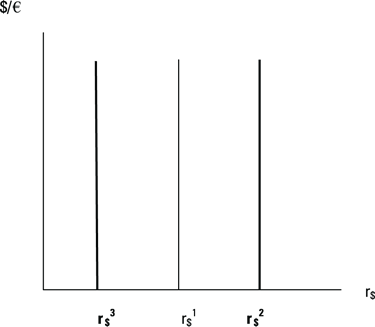
Figure 6-12: Changes in real returns on the dollar-denominated security.

In Figure 6-12, r$2 indicates a higher real return on the dollar-denominated security. You can think about the following reasons for an increase in the real return of the dollar-denominated security:

An increase in the real interest rate is consistent with a higher level of U.S. output. Everything else constant, a higher U.S. real GDP increases the money demand curve, resulting in a higher real interest rate.

A higher real interest rate is also consistent with the short-run implication of a decline in the nominal money supply or a contractionary monetary policy. Note that the money market goes back to its initial position as the price level declines in the long run. Therefore, if the source of the shock lies in monetary policy, the real interest rate goes down to its initial level both in the money market and in the foreign exchange market (r$1).

Also in Figure 6-12, r$3 shows a lower real return on the dollar-denominated security. These are the possible reasons for the decline in real returns from r$1 to r$3:

A decline in the real interest rate is consistent with a lower level of U.S. output. Everything else constant, a lower output decreases the money demand curve, resulting in a lower interest rate.

A lower real interest rate is also consistent with the short-run implication of an increase in the nominal money supply or an expansionary monetary policy. Again, the money market goes up to its initial position as the price level increases in the long run. Therefore, the real interest rate goes back to its initial level both in the money market and in the foreign exchange market (r$1).

Equilibrium in the foreign exchange market

Time to find our equilibrium! Now you can integrate the downward-sloping parity curve (expected real return on the euro-denominated security in dollars) and the perfectly inelastic curve (real return on the dollar-denominated security) into the asset approach to exchange rate determination. Figure 6-13 indicates the determination of the equilibrium exchange rate based on the MBOP.

Point 1 in Figure 6-13 shows the equilibrium exchange rate (ER1), where the real return on the dollar-denominated security equals the expected real return on the euro-denominated security (r$=r€E). At this point, you, the investor, are indifferent between the dollar- and euro-denominated securities.

Figure 6-13: Foreign exchange market (MBOP).

How do we know that the foreign exchange market settles at the exchange rate ER1 at Point 1? Suppose that, for some reason, the market isn’t in equilibrium, and the current exchange rate is ER2. The associated point (Point 2) on the downward-sloping parity curve indicates that the expected real return on the euro-denominated deposit is less than that on the dollar-denominated security. As an investor, you’re then inclined to sell your euros, buy dollars, and invest in the dollar-denominated security. The dollar appreciates, bringing the foreign exchange market equilibrium to Point 1.

Similarly, if the current exchange rate is ER3, Point 3 indicates that the expected real return on the euro-denominated security is now higher than the real return on the dollar-denominated security. In this case, as an investor, you sell your dollars, buy euros, and invest in the euro-denominated security. The dollar depreciates, and the equilibrium in the foreign exchange market returns to Point 1.

In summary, when the parity condition holds, there’s no excess supply of or excess demand for any security. Therefore, the foreign exchange market is in equilibrium when the parity condition holds. Investors are indifferent between dollar- and euro-denominated securities.

Changes in the foreign exchange market equilibrium

When you look at Figure 6-13, keep in mind that a number of money market-related variables in either the U.S. or the Euro-zone can change the equilibrium exchange rate. Following are some examples of the variables that can change the equilibrium:

The U.S. money market–related variables: Figure 6-14 shows both an increase and a decrease in the real return on the dollar-denominated security (r$2 and r$3, respectively).

Figure 6-14: Shocks in the U.S. money market and the exchange rate.

• An increase in the real return on the dollar-denominated security (r$2) may be the result of an increase in the money demand curve, due to an increase in the U.S. output or the short-run result of a decline in the nominal money supply. The changes in the money market that lead to a higher real return on the dollar-denominated security are associated with an appreciation of the dollar (ER2).

• Conversely, a decline in the real return on the dollar-denominated security (r$3) may be the result of decline in the money demand curve, due to a decline in the U.S. output or the short-run result of an increase in the nominal money supply. These changes lead to the depreciation of the dollar (ER3).

The Euro-zone’s money market-related variables: In Figure 6-15, the downward-sloping parity curve shows the expected real return on the euro-denominated security. You know that this curve implies the money market conditions in the Euro-zone and is defined by the right side of the parity equation:

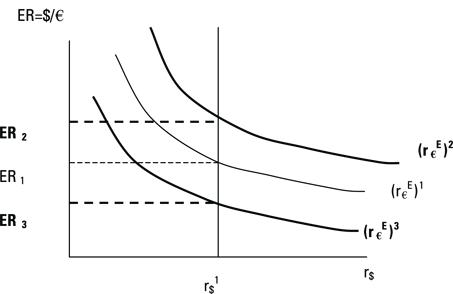
Figure 6-15: Shifts in the parity condition and the exchange rate.

In the following equation, r€ indicates the real interest rate in the Euro-zone’s money market. As in the case of the U.S. money market, a change in the money demand or supply in the Euro-zone can change the real return on the euro-denominated security.

• In Figure 6-15, (r€E)2 indicates an increase in the parity curve. The reason for this shift can be an increase in the real interest rate in the Euro-zone (r€). Either an increase in the Euro-zone’s output or the short-run effect of a decline on the nominal money supply increases the real interest rate in the Euro-zone and, therefore, increases the parity curve. This increase in the parity curve is associated with the depreciation of the dollar (ER2) compared to the initial exchange rate (ER1).

• Again in Figure 6-15, (r€E)3 indicates a decline in the parity curve, which is related to a decline in the real interest rate of the Euro-zone. Either a decline in the Euro-zone’s output or the short-run effect of an increase in the nominal money supply decreases the Euro-zone’s real interest rate. The previous equation indicates that such a decline decreases r€, thereby decreasing the parity curve, which leads to an appreciation of the dollar (ER3) compared to the initial exchange rate (ER1).

For now, don’t change the expected exchange rate in the bracket. That change happens in Chapter 7.

Combining the Money Market with the Foreign Exchange Market

This section discusses the capability to combine the money market and the foreign exchange market in the MBOP. Combining the two makes it possible to relate the change in the money market of one of the countries to the changes in the exchange rate.

The combined MBOP

At the beginning of this chapter, I mentioned that the MBOP model combines two models: the money market and the foreign exchange market. Figure 6-16 shows the combined MBOP model.

The combination of the money market and the foreign exchange market is possible because the y-axis of the U.S. money market (the real interest rate in the U.S.) is the same as the x-axis of the foreign exchange market (the real return on the dollar-denominated security). Note that the U.S. money market is rotated to take advantage of the common axes in separate models. Also note that Figure 6-16 explicitly shows the U.S. money market. The Euro-zone’s money market is implied by the parity curve in the foreign exchange model (r€E).

Figure 6-16 also makes it clear that, according to the MBOP, the exchange rate observed in the foreign exchange market has to be consistent with the money market equilibrium in both the U.S. and Euro-zone money markets. In other words, the current exchange rate observed on the y-axis of the foreign exchange market is determined based on the real return on the dollar- and euro-denominated securities. Of course, the real return on the euro-denominated security is transformed into the expected real return on the euro-denominated security in dollars so that the real returns on these two different securities are comparable.

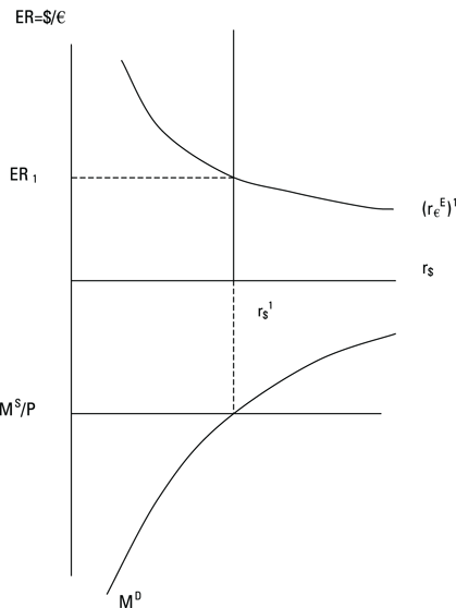
Figure 6-16: The combined MBOP.

Changes in the exchange rate equilibrium in the combined MBOP

The variables that affect the current exchange rate remain the same as discussed in the previous section. The only difference in Figure 6-16 is that you can see the U.S. money market explicitly, and the Euro-zone’s money market is implied by the parity curve in the foreign exchange market.

Therefore, shocks to output or nominal money supply (the latter has an effect only in the short run) either in the U.S. or the Euro-zone money market change the way investors compare dollar- and euro-denominated securities.

Chapter 7 provides examples for short- and long-run effects of changes in two countries’ money markets on the current exchange rate.

Keeping It Straight: What Happens When You Use a Different Exchange Rate?

You must decide which money market you want to indicate as the explicit money market or which exchange rate you want to use in the MBOP. However, be careful about a few points so that the explicit money market correctly lines up with the exchange rate.

Consider Figure 6-16, in which the U.S. money market is the explicit money market:

If you want to show the U.S. money market as the explicit money market, know that the y-axis of the money market becomes the x-axis of the foreign exchange market. Therefore, the real interest rate in the U.S. or the real return on the dollar-denominated security becomes your y-axis in the money market and your x-axis in the foreign exchange market.

If the x-axis of the foreign exchange market is in dollars, you have to express the exchange rate on the y-axis in dollars as well. Therefore, you use the dollar–euro exchange rate. In this case, the downward-sloping parity curve in the foreign exchange market shows the expected real return on the euro-denominated security and, therefore, indicates the money market conditions in the Euro-zone.

Again, consider Figure 6-16. You can also start with the decision of which exchange rate to use:

If you want to use the dollar–euro exchange rate, the x-axis of the foreign exchange model has to be in dollars, indicating the real returns in dollars. Because the x-axis of the foreign exchange model implies the y-axis of the money market, the money market must indicate the U.S. money market. Therefore, the downward-sloping parity curve in the foreign exchange market shows the Euro-zone’s money market.

Figure 6-17 gives a different example of a combined MBOP. Apply the previously mentioned considerations (in the bulleted list) to this figure.

In this model, the exchange rate is defined as the Australian dollar–dollar rate (A$/$). Thus, you must keep the foreign exchange market in Australian dollars. Therefore, the x-axis of the foreign exchange model must imply the real returns on the Australian dollar-denominated security. Because the x-axis of the foreign exchange model becomes the y-axis of the money market, the explicit money market shows the Australian money market. In this case, the downward-sloping parity curve in the foreign exchange market indicates the monetary policy of the U.S.

Figure 6-17: Keeping it straight.