
Chapter 4
It’s All about Change: Changes in the Exchange Rate
In This Chapter
![]() Observing changes in selected exchange rates
Observing changes in selected exchange rates
![]() Observing the relationship between changes in exchange rates and macroeconomic fundamentals
Observing the relationship between changes in exchange rates and macroeconomic fundamentals
![]() Developing a visual understanding of exchange rate regimes
Developing a visual understanding of exchange rate regimes
If you like visualizing concepts, you’re in luck! This chapter is all about visualizing changes in exchange rates. Using example exchange rates, we look at how these rates fluctuate over time. Through these examples, you get a good look at the highly volatile nature of exchange rates.
Changes in exchange rates cause you to ask why these changes are happening. You can find the reasons behind why exchange rates change in Chapters 5, 6, and 7. In this chapter, graphs showcase the actual changes in selected exchange rates. In addition to exchange rates, the graphs include macroeconomic fundamentals, including GDP growth, inflation rates, and interest rates. The purpose of this chapter is to introduce a visual approach to the relationship between changes in exchange rates and macroeconomic fundamentals without providing a theory-based discussion.
In this chapter, I use the terminology introduced in Chapter 2, including such terms as percent change in the exchange rate, appreciation, and depreciation. This chapter really serves as a bridge between the definition- and calculation-oriented Chapters 2 and 3 and the upcoming Chapters 5, 6, and 7, which represent the theories of exchange rate determination.
Also in this chapter, you start developing some sensitivity to exchange rate regimes, at least in a visual context. Chapters 11, 12, and 13 focus on the extent of government/central bank interventions in exchange rates, so this chapter prepares you to ask questions regarding exchange rate regimes when you have exchange rate data.
Considering a Visual Approach to Changes in Exchange Rates
Exchange rates behave differently over time. The example exchange rates in this chapter certainly prove this point. I use the Japanese yen–dollar and Indonesian rupiah–dollar exchange rates as example exchange rates for this chapter. The Chinese yuan–dollar exchange rate appears in the section on exchange rate regimes.
 This section uses the yen–dollar and the rupiah–dollar exchanges rates as example exchange rates. As Chapter 2 discusses, an increase in these exchange rates implies the depreciation of the yen or the rupiah against the dollar. In addition to using exchange rates in levels, sometimes you see the percent change in exchange rates. If the sign of the percent change is positive, (for example, in the yen–dollar rate), you can express the depreciation in the yen as a percentage. If the sign is negative, it indicates the percent change of appreciation in the yen.
Figure 4-1 shows the quarterly nominal yen–dollar exchange rate for more than 40 years. The general trend is downward sloping, which means a gradual appreciation in the yen against the dollar. The data suggest that the exchange rate in the first quarter of 1970 was ¥360 per dollar and that it declined to ¥77.4 per dollar in the fourth quarter of 2011. Of course, you observe fluctuations around the downward trend. For example, during the mid-1970s and 1980s, the yen depreciated against the dollar.
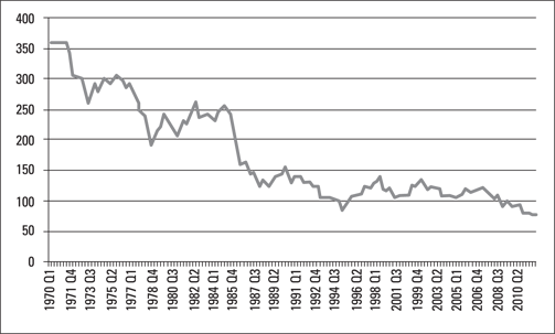
Notes: International Financial Statistics of the IMF. Data are available at www.imf.org.
Figure 4-1: The yen–dollar quarterly nominal exchange rates (1970:Q1 to 2011:Q4).
Because the nominal effective and real effective exchange rate data are available for Japan, you can inspect them in Figure 4-2. In terms of the yen–dollar exchange rate, the real effective or trade-weighted exchange rates indicate the cost of the Japanese consumption basket to the weighted average cost of the consumption basket associated with Japan’s major trade partners. Figure 4-2 shows effective exchange rates in both nominal (not adjusted for inflation) and real (adjusted for inflation) terms. It also indicates that, between 1980 and the mid-1990s, the purchasing power of the Japanese yen steadily increased. Following a decline in the early and mid-2000s, both the nominal effective and real effective yen–dollar rates increased again until late 2011.
When you compare Figures 4-1 and 4-2, keep in mind that Figure 4-1 shows the nominal yen–dollar exchange rate, whereas Figure 4-2 indicates the nominal effective and real effective rates involving the yen and a basket of currencies that consists of the currencies of Japan’s major trade partners. In Figure 4-1, you observe that the yen gradually appreciated against the dollar during the period under consideration (1970:Q1 to 2011:Q4). Based on this figure, you can conclude that, over the years, smaller amounts of yen were required to buy one dollar. Actually, Figure 4-2 expresses something similar, where the comparison isn’t between only two currencies, but is between the yen and the currencies of Japan’s major trade partners. The rising nominal effective rate means an appreciation of the yen against the basket of currencies. The rising real effective exchange rate shows that, even if you include the cost of the Japanese consumption basket and other countries’ consumption baskets in the calculation, the yen appreciated against the currencies of Japan’s major trade partners.
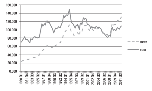
Notes: International Financial Statistics of the IMF. The consumer price index of Japan and its trade partners are used to calculate the indices. Data are available at www.imf.org.
Figure 4-2: The nominal and real effective exchange rate index for Japan, 2005=100 (1980:Q1 to 2011:Q4).
Another example exchange rate is the rupiah–dollar rate. Because the nominal effective and real effective exchange rates aren’t available for this currency, you observe only the changes in the nominal rupiah–dollar exchange rate in Figure 4-3.
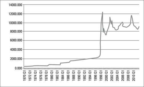
Notes: International Financial Statistics of the IMF. Data are available at www.imf.org.
Figure 4-3: The nominal Indonesian rupiah–dollar exchange rate (1970:Q1 to 2011:Q4).
The figure starts with Rp326 per dollar in 1970:Q1, and the rate only slightly depreciates until 1971:Q4. At the beginning of the graph, you see a straight line, which reflects the lack of change in the rupiah–dollar exchange rate between 1971:Q4 and 1978:Q3. During this period, the rupiah–dollar exchange rate remained as Rp415 per dollar. Then you observe a steady depreciation of the rupiah approaching Rp1,644 per dollar in 1986:Q4, which continued until 1997:Q3, when the rate reached Rp2,791 per dollar. Next quarter, 1997:Q4, the rupiah–dollar rate increased to Rp4,005, indicating an almost 44 percent depreciation in the rupiah. But worse was yet to come. Next quarter, 1998:Q1, the rupiah increased even further to Rp9,433, which implied a 136 percent depreciation in the rupiah against the dollar. Finally, the exchange rate reached Rp12,252 in 1998:Q3.
 These large deprecations of the Indonesian rupiah took place during the Asian crisis of 1997–1998, a currency crises that involved several Asian countries. Chapter 13 examines the Asian crisis and the reasons for currency crises in general.
Looking at How Macroeconomic Variables Affect Exchange Rates
This section provides a visual approach to changes in exchange rates by introducing graphs that capture changes in exchange rates along with changes in the selected macroeconomic fundamentals. The yen–dollar and rupiah–dollar rates continue to be the example exchange rates. Note that upcoming graphs show the change in the exchange rate and the change in Japan’s and Indonesia’s fundamentals, such as real GDP growth rates, inflation rates, and interest rates.
This section doesn’t go into a deep discussion of exchange rate determination. Chapters 5, 6, and 7 cover macroeconomic variables that explain the changes in exchange rates.
Understanding the limitations of this section is important. Clearly, when considering an exchange rate, you must consider two countries’ fundamentals (as with the U.S. and Japan or the U.S. and Indonesia, for example). The formal treatment of exchange rate determination in Chapters 7 and 8 examines the change in the exchange rate and the difference between two countries’ inflation and interest rates. In this chapter, matters are simpler. Additionally, focusing on the macroeconomic fundamentals of Japan and Indonesia makes sense because of the relatively slower changes in the fundamentals of the U.S. Therefore, you see the change in exchange rates and Japan’s and Indonesia’s fundamentals, but not fundamentals of the U.S..
Output and exchange rates
Just to clarify the terminology, output refers to a country’s real gross domestic product (GDP). Because real GDP is adjusted for the changes in inflation (in other words, it has no price effect in it), it can also be referred to as output. The relationship between exchange rates and output, usually the percent change in output (in short, growth rates), is used. Some of the exchange rate determination theories, such as the monetary approach to exchange rates (see Chapter 7), predict that higher growth rates in a country lead to an appreciation of this country’s currency.
Figure 4-4 illustrates the relationship between percent change in the yen–dollar exchange rate and growth rates in Japan’s real GDP. One striking aspect of Figure 4-4 is that the exchange rate is more volatile than output. You observe that the changes in the exchange rate are much larger than the changes in output. In terms of the expected relationship between changes in the exchange rate and economic growth, some periods, such as the early 1980s, show appreciation of the yen when growth rates are higher and show depreciation of the yen when the growth rates are lower. These associations are consistent with the predictions of the theory that Chapters 6 and 7 cover (the Monetary Approach to Balance of Payments, or the MBOP). However, when you look at the early quarters of 2010, you observe an appreciation of the yen accompanied by slower growth rates.

Notes: International Financial Statistics of the IMF. cher and chrgdp indicate the percent change in the exchange rate and growth rate of real GDP, respectively. Data are available at www.imf.org.
Figure 4-4: Percent change in the yen–dollar exchange rate and real GDP growth rates in Japan (1980:Q1 to 2011:Q4).
Another example of the exchange rate output relationship is the rupiah–dollar rate and growth rate of Indonesia’s real GDP. Figure 4-5 depicts this relationship. The data availability in the real GDP is the reason the figure starts in 1998:Q1. This figure is interesting because of the spike in the exchange rate, which indicates a 136 percent depreciation in the rupiah after the Asian crisis hit Indonesia (1998:Q1). The corresponding decline in output reached about 18 percent in 1998:Q4. This observation is certainly an outlier. (You call an observation an outlier if it has a much higher or lower value than the surrounding observations.) Still, it confirms the expected relationship between depreciation in the rupiah and slower growth rates in Indonesia.
Although observing such outliers as a 136 percent depreciation in the rupiah is interesting, they make seeing the relationship between the exchange rate and the growth rate difficult for the rest of the available period. Therefore, Figure 4-6 takes out the outlier and starts with the post–Asian crisis period. Now you can better see the changes in the exchange rate and growth rates during the post-crisis period. Again, you observe a higher volatility in the rupiah–dollar exchange rate than that of the GDP growth rate. In terms of the relationship between changes in the exchange rate and GDP growth rate, the first couple quarters in 1999 and 2002, as well as in late 2004 and 2009, indicate the appreciation of the rupiah and higher growth rates. Almost 20 percent depreciation in the rupiah in the fourth quarter of 2008 coincides with declining growth rates, which confirms the theory’s expectations.
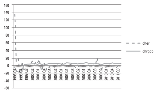
Notes: International Financial Statistics of the IMF. cher and chrgdp indicate the percent change in the exchange rate and the real GDP growth rate, respectively. Data are available at www.imf.org.
Figure 4-5: Percent change in the rupiah–dollar exchange rate and real GDP growth rates in Indonesia (1998:Q1 to 2011:Q4).
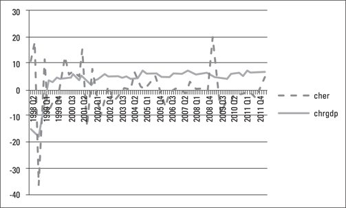
Notes: International Financial Statistics of the IMF. cher and chrgdp indicate the percent change in the exchange rate and the real GDP growth rate, respectively. Data are available at www.imf.org.
Figure 4-6: Percent change in the rupiah–dollar exchange rate and real GDP growth rates in Indonesia (1998:Q2 to 2011:Q4).
Inflation rates and exchange rates
Most theories of exchange rate determination (see Chapters 5, 7, and 9) predict depreciation in the higher-inflation country’s currency. Inflation refers to an increase in the average price level of a country, which is frequently measured by the consumer price index (CPI). Figure 4-7 shows the change in the yen–dollar exchange rate and the change in the Japanese CPI. Again, you can see higher volatility in the exchange rate compared to changes in the consumer price index.

Notes: International Financial Statistics of the IMF. cher and chcpi indicate the percent change in the exchange rate and the consumer price index, respectively. Data are available at www.imf.org.
Figure 4-7: Percent change in the yen–dollar exchange rate and the consumer price index in Japan (1970:Q2 to 2011:Q4).
In terms of the relationship between the exchange rate and the inflation rate, certainly the observation in 1974 is consistent with the theory’s expectation: As the inflation rate approached 25 percent, you observe a depreciation of the yen about 5 percent. As another example, in 1986, as the inflation rate declined, you observe an appreciation of the yen approaching 15 percent.
Figure 4-8 shows the relationship between the change in the rupiah–dollar exchange rate and the inflation rate in Indonesia. Again, the spike in the exchange rate and the inflation rate indicates the Asian crisis. The 136 percent depreciation in the rupiah in 1998:Q1 was accompanied by higher inflation rates that reached 78 percent in 1998:Q4.

Notes: International Financial Statistics of the IMF. cher and chcpi indicate the percent change in the exchange rate and the consumer price index, respectively. Data are available at www.imf.org.
Figure 4-8: Percent change in the rupiah–dollar exchange rate and the consumer price index in Indonesia (1970:Q2 to 2011:Q4).
Because of the outliers associated with the Asian crisis, seeing the relationship between changes in the exchange rates and the inflation rates is difficult. Therefore, Figures 4-9 and 4-10 indicate the pre– and post–Asian crisis periods, respectively. In Figure 4-9, spikes in the change of the exchange rates indicate major depreciations, reaching almost 40 percent in the early 1980s. They’re accompanied by higher inflation rates. However, the relationship between changes in the exchange rates and inflation rates is almost nonexistent during the 1970s and the late 1980s and 1990s. The last section of this chapter returns to these periods and provides an explanation.
Figure 4-10 shows the changes in the rupiah–dollar exchange rate and inflation rates in Indonesia during the post–Asian crisis period. Higher inflation rates and depreciation in the rupiah coincide during the later quarters of 2001, the early quarters of 2004, the later quarters of 2005 and 2008, and the early quarters of 2010. Lower inflation rates and appreciation in the rupiah coincide with the early quarters of 2002 and 2003. However, in early 2006, although the inflation rate is above 15 percent, the rupiah appreciates more than 5 percent. This result is inconsistent with the theories in Chapters 5, 6, and 7.

Notes: International Financial Statistics of the IMF. cher and chcpi indicate the percent change in the exchange rate and the consumer price index, respectively. Data are available at www.imf.org.
Figure 4-9: Percent change in the rupiah–dollar exchange rate and the consumer price index in Indonesia (1970:Q2 to 1997:Q4).

Notes: International Financial Statistics of the IMF. cher and chcpi indicate the percent change in the exchange rate and the consumer price index, respectively. Data are available at www.imf.org.
Figure 4-10: Percent change in the rupiah–dollar exchange rate and the consumer price index in Indonesia (1999:Q2 to 2011:Q4).
Interest rates and exchange rates
All exchange rate determination theories refer to the effect of interest rates on exchange rates. Chapters 5–8 discuss the effects of interest rates on the changes in exchange rates. As these chapters make clear, some theories deal with nominal interest rates, and some deal with real interest rates.
In general, nominal variables include the price effect. Real variables are adjusted for changes in prices.
The relationship between the nominal interest rate and the real interest rate is described thus:
![]()
Here r, R, and π denote the real interest rate, the nominal interest rate, and the inflation rate, respectively. This equation implies that the real interest rate is calculated by subtracting the inflation rate from the nominal interest rate. Keep in mind that real interest rates may be negative if inflation rates are higher than nominal interest rates. Upcoming figures have examples of negative real interest rates.
Because nominal interest rates are expected to increase with higher inflation rates, some of the theories in upcoming chapters (for example, see Chapter 8) predict that higher nominal interest rates in a country are consistent with the depreciation of this country’s currency. Other theories (see Chapters 5, 6, and 7) work with real interest rates and predict that higher real interest rates in a country are consistent with the appreciation of this country’s currency. Therefore, the graphs in this section show both real and nominal interest rates.
The example currencies are still the Japanese yen and the Indonesian rupiah. Because data availability on interest rates varies among countries, the following graphs show the Treasury bill (T-bill) rate in Japan and the discount rate in Indonesia.
In Figure 4-11, you can observe the change in the yen–dollar exchange rate and the nominal T-bill rates. Again, the volatility of the exchange rate is higher than that of the T-bill rates. Especially during the mid- and late 1970s, higher nominal interest rates coincide with the depreciation of the yen. However, this relationship seems to break down starting in the mid-1990s when the interest rates remained very low, but the yen–dollar rate fluctuates substantially.

Notes: International Financial Statistics of the IMF. cher and tbrate indicate the percent change in the exchange rate and the interest rate on the Japanese Treasury bill rate, respectively. Data are available at www.imf.org.
Figure 4-11: Percent change in the yen–dollar exchange rate and the Treasury bill rate in Japan (1970:q2 to 2011:q4).
Figure 4-12 indicates the relationship between changes in the yen–dollar exchange rate and the real T-bill rate in Japan. In 1974, lower (in fact, negative) real interest rates are consistent with the depreciation of the yen. Although exceptions do exist, during the 1980s and 1990s, higher real interest rates are associated with the appreciation of the yen.
In Indonesia, the graph data starts in 1990:Q1, indicating the data availability in the Indonesian discount rate. Figures 4-13 and 4-14 show the nominal and real discount rates in Indonesia, respectively. In both graphs, the Asian crisis appears as an outlier again. Figure 4-13 shows that higher nominal discount rates are associated with the depreciation of the rupiah. Figure 4-14 indicates that, in late 1998, in the aftermath of the Asian crisis, as the rupiah was depreciating, the real discount rate declined and reached almost –40 percent.
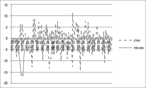
Notes: International Financial Statistics of the IMF. cher and rtbrate indicate the percent change in the exchange rate and the real interest rate on the Japanese Treasury bill rate, respectively. The inflation rate used in the calculation of the real Treasury bill rate is determined based on the percent change in the consumer price index of Japan. Data are available at www.imf.org.
Figure 4-12: Percent change in the yen–dollar exchange rate and the real Treasury bill rate in Japan (1970:q2 to 2011:q4).

Notes: International Financial Statistics of the IMF. cher and drate indicate the percent change in the exchange rate and the discount rate in Indonesia, respectively. Data are available at www.imf.org.
Figure 4-13: Percent change in the rupiah–dollar exchange rate and the discount rate in Indonesia (1990:q1 to 2011:q4).

Notes: International Financial Statistics of the IMF. cher and rdrate indicate the percent change in the exchange rate and the real discount rate in Indonesia, respectively. Data are available at www.imf.org.
Figure 4-14: Percent change in the rupiah–dollar exchange rate and the real discount rate in Indonesia (1990:q1 to 2011:q4).
Because the outliers associated with the Asian crisis make it difficult to observe the relationship between the interest rate and the exchange rate, Figures 4-15 and 4-16 show the nominal and real discount rates, as well as changes in the rupiah–dollar exchange rate during the pre- and post-crisis periods, respectively.
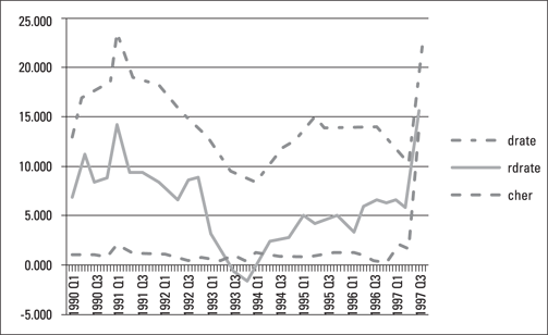
Notes: International Financial Statistics of the IMF. cher, drate, and rdrate indicate the percent change in the exchange rate, the nominal discount rate, and the real discount rate in Indonesia, respectively. Data are available at www.imf.org.
Figure 4-15: Percent change in the rupiah–dollar exchange rate and the nominal and real discount rates in Indonesia during the pre-crisis period (1990:Q1 to 1997:Q4).

Notes: International Financial Statistics of the IMF. cher, drate, and rdrate indicate the percent change in the exchange rate, the nominal discount rate, and the real discount rate in Indonesia, respectively. Data are available at www.imf.org.
Figure 4-16: Percent change in the rupiah–dollar exchange rate and the nominal and real discount rates in Indonesia during the post-crisis period (1999:Q3 to 2011:Q4).
Figure 4-15 covers the pre–Asian crisis period. Still, you can clearly see the start of the Asian crisis, indicated by the large depreciation of the rupiah that starts in the second quarter of 1997. Except for the decline in the nominal and real discount rates in 1993 (in fact, the real discount rate was negative in late 1993), the nominal and real discount rates were positive. The fact that you see only small changes in the exchange rate during the pre–Asian crisis period is related to government interventions in the exchange rate, which the last section of this chapter touches on.
Figure 4-16 shows that the rupiah–dollar exchange rate fluctuated more during the post-crisis period. Nominal interest rates were declining, and real interest rates were fluctuating more in this period. Larger depreciations took place in early 2001 and late 2008, when the real interest rates were declining and negative, respectively. Largest appreciations happened in late 2001, early 2002, mid-2003, mid-2009, and early 2011, all accompanied by higher real interest rates. However, in early 2006, an appreciation of about 7 percent took place when the real discount rate was –5 percent. This scenario isn’t consistent with the theories in Chapters 5, 6, and 7.
Uncovering Hidden Information in Graphs: Exchange Rate Regimes
Governments or central banks may intervene in the exchange rate. Chapter 13 discusses such interventions in detail. Still, you can start thinking about this subject now, at least to recognize such interventions on graphs.
Some of the graphs in this chapter show some odd observations. Sometimes an exchange rate is highly volatile, but then in some periods, it seems to be changing only slowly or it remains the same for a number of years. This section refers to some of the previous graphs in this chapter and examines them again to see whether they imply any information about government interventions in exchange rates. In addition to Japan and Indonesia, China is added to this section’s discussions on exchange rate regimes.
Defining exchange rate regime
The exchange rate between two currencies may be determined in international foreign exchange markets or in a government office. If an exchange rate — say, the yen–dollar rate — is determined in international foreign exchange markets based on the demand for and supply of the yen, then the markets determine the exchange rate. This situation is similar to the case of any other good, such as oranges, whose price is determined in the market based on the demand for and supply of oranges. If the exchange rate is mainly determined in international foreign exchange markets, it’s called a floating exchange rate regime.
Exchange rates involving developed countries’ currencies, such as the U.S. dollar, the euro, the pound, the yen, and the Swiss franc, are determined in foreign exchange markets — mostly. When referring to these currencies, you may hear the term dirty float because of occasional central bank interventions in foreign exchange markets.
If floating or dirty floating currencies are at one extreme of the foreign exchange regime spectrum, pegged exchange rate regimes are toward the other end of the spectrum. In a pegged exchange rate regime, governments either don’t allow their currency to be traded in international foreign exchange markets or impose restrictions on trade. In fact, governments determine the exchange rate unilaterally and announce it to the world. Although a variety of pegged exchange rate regimes exist, for the purpose of this chapter, you can think about pegged regimes in which the government determines the exchange rate. As Chapter 13 indicates, governments have reasons to keep the exchange rate involving the domestic currency at a certain level.
 Don’t think of pegging the exchange rate as an easy decision. As any other decision, the decision to peg implies tradeoffs. Governments that decide to peg their currency have to decide whether they want to allow foreign portfolio investment in and out of the country. If governments allow foreign portfolio investment, this approach attracts foreign investors into the country and opens new sources of financing for the country. But it can also spark a currency crisis, as foreign investors cash out their investment in the fear of depreciation, leaving the country in desperate need of foreign currency. Alternatively, a government may decide to peg the exchange rate without allowing foreign portfolio flows. This approach may prevent a currency crisis, but it also makes an additional financing opportunity unavailable.
Visualizing exchange rate regimes
The yen has been a floating currency for almost four decades. Figure 4-1 shows a straight line at the beginning of the data, where the yen–dollar exchange rate seems to remain the same. In fact, the data shows that the yen–dollar exchange rate remained as ¥360 per dollar between 1970:Q1 and 1971:Q2. It’s highly unlikely for an exchange rate to remain the same if the currency is almost freely exchanged in international foreign exchange markets. When you look at the exchange rate data earlier than 1970, you see periods of unchanging exchange rates. It seems that Japan did what China is now doing. Before the mid-1970s, Japan pegged its exchange rate with the dollar (and other major currencies of that time) to enhance its export performance.
 Assuming away transportation and other costs, a shipment of ¥100,000 costs about $278 to American consumers at the exchange rate of ¥360 per dollar. Suppose the yen appreciates to ¥300. In this case, the same shipment costs $333. With everything else constant, Japan can export more to the U.S. when the peg of the yen implies a lower value of the yen.
A similar situation exists in terms of the rupiah–dollar exchange rate in Figure 4-3. The data starts with Rp326 in 1970:Q1 and only slightly depreciates until 1971:Q4. At the beginning of the graph, you see a straight line, which reflects no change in the rupiah–dollar exchange rate between 1971:Q4 and 1978:Q3. During this period, the rupiah–dollar exchange rate remained as Rp415 per dollar. Then you observe a notable steady depreciation of the rupiah, approaching Rp1,644 per dollar in 1986:Q4. A steady depreciation took place until 1997:Q3, where the rate reached Rp2,791 per dollar.
You can make two observations about Figure 4-3. First, after the Asian crisis, Indonesian governments seem to have stopped pegging the rupiah because the exchange rate fluctuates more during the post-crisis period.
The second observation of Figure 4-3 isn’t visible on the graph, but you can discover it by reading about Indonesia’s approach to economic development. Until the mid-1980s, the slowly depreciating rupiah reflected a policy similar to the one Japan followed in earlier decades: improving export performance by keeping the rupiah–dollar rate relatively high. In the mid-1980s, the Indonesian government pegged its currency for a different reason. Many developing countries, including Indonesia, recognized the limited financing opportunities associated with exports. They wanted to attract portfolio investment into their countries, which involved foreign investors buying, for example, rupiah-denominated securities (bonds, stocks, and so on). Again, Chapter 13 provides a detailed discussion of these changes in policies and their consequences.
Finally, you can refer to Figure 2-4 in Chapter 2 to see the yuan–dollar exchange rate. As the figure indicates, China has pegged the yuan in accordance with its development policy. Building an industrial base through imports of equipment may have been important to China until the mid-1990s. When China achieved this industrial base, the country’s export performance became more important to Chinese policymakers. Then the aim shifted to improving export performance by undervaluing the yuan.
The yuan–dollar exchange rate was as low as CNY1.71 per dollar in 1981, compared to its highest point of CNY8.64 in 1994. The Chinese government tried to keep the yuan overvalued at CNY1.71, to make imports cheaper. Suppose that China wanted to import $100,000 worth of industrial equipment from the U.S., assuming away all transportation and other costs. At the exchange rate of CNY1.71, this shipment costs China CNY171,000 ($100,000 × CNY1.71). However, if the exchange rate is, say CNY8.64, the same shipment costs CNY864,000 ($100,000 × CNY8.64). Undervaluation of the yuan at the level of CNY8.64 is helpful to improve China’s export performance because the dollar price of a CNY100,000 shipment is $58,479 at CNY1.71 (CNY100,000 ÷ 1.71) and $11,574 at CNY8.64 (CNY100,000 ÷ 8.64).
Also in Figure 2-4, the slight revaluation since 2006 is indicative of the limited success of developed countries such as the U.S., which have complained about China’s extensive use of foreign exchange control to improve its export performance.