
Surface Topography Characterisation
Richard Leach
This chapter discusses the field of surface topography characterisation, i.e. the analysis of the measurement data from surface topography measuring instrumentation. The field is introduced with a brief history. Profile and areal characterisation are both covered in detail including the basic concepts, filtering methods and surface texture parameters. In the areal case, both field and feature parameters are discussed, along with fractal methods. The still-evolving international specification standards infrastructure is covered in detail.
Keywords
Surface Topography Characterisation; Profile Characterisation; Areal Characterisation; Filtering; Surface Texture Parameters; Field Parameters; Feature Parameters; Fractal Methods
8.1 Introduction to surface topography characterisation
The characterisation of surface topography is a complicated branch of metrology with a large range of parameters available. Surface form characterisation has been covered elsewhere [1], and this book concentrates on surface texture characterisation, that is to say the handling of surface texture data to give meaningful information once a measurement has been made. The measurement of freeform surfaces is also a subject area in itself and is covered in detail elsewhere [2]. The proliferation of surface texture characterisation parameters has been referred to as ‘parameter rash’ [3] – at any one time there can be over 100 parameters to choose from. However, due to recent activities, there is now a coherent international standards infrastructure to support surface texture characterisation. Profile characterisation has been standardised for some time now, and areal specification standards are now available.
The first important work on areal surface texture was carried out by a European project led by Ken Stout, then from the University of Birmingham [4]. This project ended with the publication of the ‘Blue Book’ [5] and the definition of the so-called Birmingham-14 parameters. Following this project, ISO started standardisation work on areal surface texture. However, ISO experts rapidly realised that further research work was needed to determine the stability of areal parameters and their correlation with the functional criteria used by industry. A further project (SURFSTAND) was carried out between 1998 and 2001, by a consortium of universities and industrial partners, led by Liam Blunt of the University of Huddersfield. SURFSTAND ended with the publication of the ‘Green Book’ [6] and generated the basic documents for forthcoming specification standards.
This chapter will summarise the surface texture characterisation methods that are now fully standardised. There are many other parameters (and filtering methods) that can be found on less recent instrumentation and in use in many industries, but this book has only considered the ISO standard methods, as these are the most likely to be the methods used in the near future. Further methods for surface characterisation, including those from the fields of roundness measurement, and frequency and waveform analysis can be found elsewhere [7–9].
Parameters for areal surface texture are relatively new, and there has been limited research on their use. For this reason, some of the areal parameters are just presented in this book as stated in the ISO specification standards with little or no description of their uses. It is also expected that most users of surface texture parameters will have access to software packages that can be used to calculate parameters and will not attempt to code the parameters from scratch. However, software packages should be checked for correctness where possible using software measurement standards (see Section 6.15). A more thorough treatment of the ISO parameters and filtering methods and a range of industrial case studies can be found elsewhere [9].
8.2 Surface profile characterisation
Surface profile measurement was described in Section 6.4. The surface profile characterisation methods that have been standardised by ISO are presented here. Section 8.4 presents some of the fractal methods that are available. There are three types of profile that are defined in ISO specification standards [10,11]. Firstly, the traced profile is defined as the trace of the centre of a stylus tip that has an ideal geometrical form (conical, with spherical tip) and nominal tracing force, as it traverses the surface. Secondly, the reference surface is the trace that the probe would report as it is moved along a perfectly smooth and flat workpiece. The reference profile arises from the movement caused by an imperfect datum guideway. If the datum were perfectly flat and straight, the reference profile would not affect the total profile. Lastly, the total profile is the (digital) form of the profile reported by a real instrument, combining the traced profile and the reference profile. Note that in some instrument systems, it is not practicable to ‘correct’ for the error introduced by datum imperfections, and the total profile is the only available information concerning the traced profile.
The above types of profile are primarily based on stylus instruments. Indeed, stylus instruments are the only instruments that are covered by ISO profile standards at the time of writing (see Section 8.2.10). However, many optical instruments allow a profile either to be measured directly (scanned) or extracted in software from an areal map. In this case, the profile definitions need to be interpreted in an appropriate manner (e.g. in the case of a coherence scanning interferometer, see Section 6.7.3.4, the reference profile will be part of the reference mirror surface).
Two more definitions are required before we can move on to filtering and surface texture parameters.
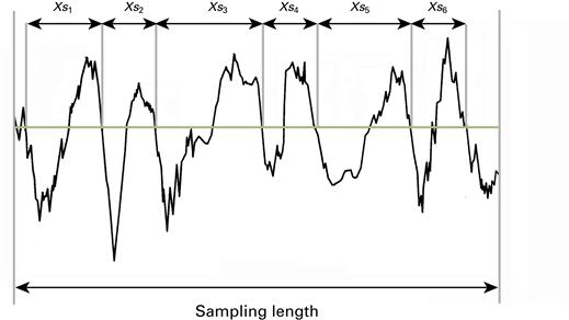
8.2.1 Evaluation length
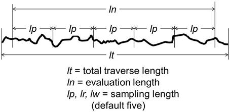
The evaluation length is the total length along the surface (x-axis) used for the assessment of the profile under evaluation. It is normal practice to evaluate roughness and waviness profiles (see Sections 8.2.3.2 and 8.2.3.3) over several successive sampling lengths, the sum of which gives the evaluation length. For the primary profile, the evaluation length is equal to the sampling length. ISO 4287 [11] advocates the use of five sampling lengths as the default for roughness evaluation, and if another number is used the assessment parameter (see Section 8.2.5) will have that number included in its symbol, for example Ra6. No default is specified for waviness. With a few exceptions, parameters should be evaluated in each successive sampling length and the resulting values averaged over all the sampling lengths in the evaluation length. Some parameters are assessed over the entire evaluation length. To allow for acceleration at the start of a measurement and deceleration at the end of a measurement (when using a stylus instrument), the instrument traverse length is normally a little longer than the evaluation length.
8.2.2 Total traverse length
The total traverse length is the total length of surface traversed in making a measurement. It is usually greater than the evaluation length due to the need to allow a short over-travel at the start and end of the measurement to allow mechanical and electrical transients to be excluded from the measurement, and to allow for the effects of edges on the filters. Figure 8.1 summarises the various lengths used for profile characterisation.
8.2.3 Profile filtering
Filtering plays a fundamental role in surface texture analysis. In this context, it is any means (usually electronic or computational, but sometimes mechanical) for selecting for analysis a range of structure in the total profile that is judged to be that of significance to a particular situation. Alternatively, it may be thought of as a means of rejecting information considered irrelevant, including, for example, attempts to reduce the effect of instrument noise and imperfections. Filters select (or reject) structure according to its scale in the x-axis, that is in terms of wavelengths or spatial frequencies. A filter that rejects short wavelengths while retaining longer ones is called a low-pass filter since it preserves (or lets pass) the low frequencies. A high-pass filter preserves the shorter wavelength features while rejecting longer ones. The combination of a low-pass and a high-pass filter to select a restricted range of wavelengths with both high regions and low regions rejected is called a band-pass filter. The attenuation (rejection) of a filter should not be too sudden else we might get very different results from surfaces that are almost identical apart from a slight shift in the wavelength of a strong feature. The wavelength at which the transmission (and so also the rejection) is 50 % is called the cut-off of that filter (note that this definition is specific to the field of surface texture).
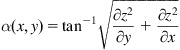
The transmission characteristics of a filter are determined by its weighting function. The weighting function, standardised in ISO 16610 part 21 [3,12], in the form of a Gaussian probability function is described mathematically by
(8.1)
 (8.1)
(8.1)
where α is a constant designed to provide 50 % transmission at a cut-off wavelength of λ and is equal to
(8.2)
The filter effect of the weighting function, s(x), is exclusively determined by the constant α. Filtering produces a filter mean line which results from the convolution of the measured profile with the weighting [3].
A surface profile filter separates the profile into long-wave and short-wave components (Figure 8.2). There are three filters used by instruments for measuring roughness, waviness and primary profiles:
1. λs profile filter
This is the filter that defines where the intersection occurs between the roughness (see Section 8.2.3.2) and shorter wavelength components present in a surface.
2. λc profile filter
This is the filter that defines where the intersection occurs between the roughness and waviness (see Section 8.2.3.3) components.
3. λf profile filter
This is the filter that defines where the intersection occurs between the waviness and longer wavelength components present in a surface.
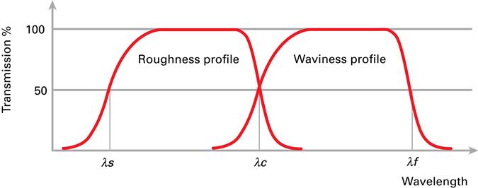
Almost all modern instruments and software packages now employ a Gaussian filter according to ISO 16610 part 21 [12]. However, older instruments may employ other forms of filter, for example the 2RC filter [3,13]. Also, many modern instruments allow so-called robust filters to be used – these are filters that are better suited to end-effects and spurious data [14,15]. It is important to be aware of the type of filter used by an instrument, and care should be taken when comparing data from older instruments to those from modern instruments.
8.2.3.1 Primary profile
The primary profile is defined as the total profile after application of the short-wavelength (low-pass) filter, with cut-off, λs, but including the effect of the standardised probe (see Section 6.6.1). Ultimately, the finite size of the stylus limits the rejection of very short wavelengths, and in practice this mechanical filtering effect is often used by default for the λs filter (similar arguments can be used throughout this chapter for optical instruments; for example, the equivalent to a finite stylus radius for an optical instrument will be either the spot size, diffraction limit or pixel spacing). Since styli vary, and since the instrument will introduce vibration and other noise into the profile signal that has equivalent wavelengths shorter than the stylus dimensions, the best practice is always to apply λs filtration upon the total profile. Figure 8.3 relates the primary to the roughness and waviness profiles.

8.2.3.2 Roughness profile
The roughness profile is defined as the profile derived from the primary profile by suppressing the long-wave component using a long-wavelength (high-pass) filter, with cut-off, λc. The roughness profile is the basis for the evaluation of the roughness profile parameters. Note that such evaluation automatically includes the use of the λf profile filter, since it derives from the primary profile.
8.2.3.3 Waviness profile
The waviness profile is derived by the application of a band-pass filter to select the surface structure at rather longer wavelengths than the roughness. Filter λf suppresses the long-wave component (profile component) and filter λc suppresses the short-wave component (roughness component). The waviness profile is the basis for the evaluation of the waviness profile parameters.
8.2.4 Default values for profile characterisation
ISO 4287 [11] and ISO 4288 [16] define a number of default values for various parameters that are used for surface profile characterisation. Unless otherwise stated these default values apply. For example, unless otherwise stated, five sampling lengths are used to calculate the roughness parameters. Table 8.1 gives the relationship between cut-off wavelength, tip radius and maximum sampling spacing. It is important to stress here that the default values are just defaults – they are not requirements. For example, if five sampling lengths would produce an evaluation length that is larger than the length of the surface available for measurement, then fewer sampling length or a smaller sampling length can be used. In each measurement case, the adherence to the default values should be considered appropriately.
Table 8.1
Relationship Between Cut-Off Wavelength, Tip Radius (rtip) and Maximum Sampling Spacing [16]
| λc (mm) | λs (μm) | Roughness Cut-Off Wavelength Ratio λc/λs | rtip max (μm) | Maximum Sampling Spacing (μm) |
| 0.08 | 2.5 | 30 | 2 | 0.5 |
| 0.25 | 2.5 | 100 | 2 | 0.5 |
| 0.8 | 2.5 | 300 | 2 | 0.5 |
| 2.5 | 8 | 300 | 5 | 1.5 |
| 8 | 25 | 300 | 10 | 5 |
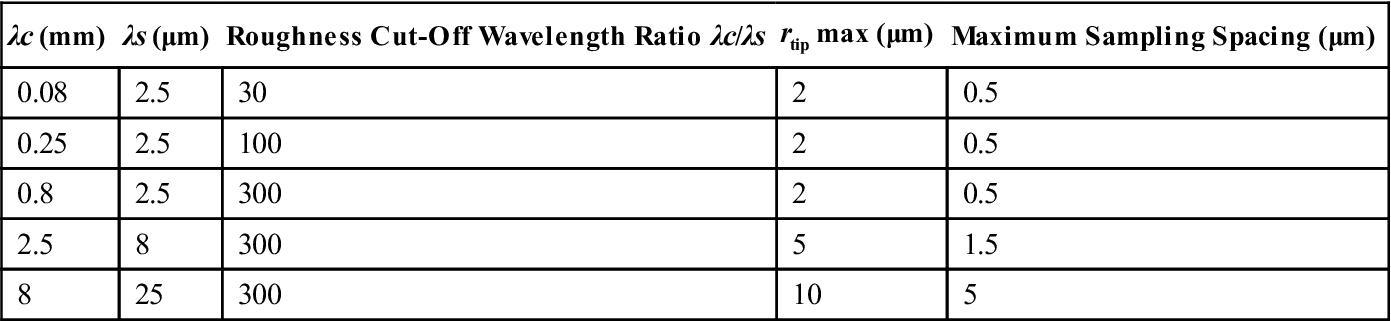
When a component is manufactured from a drawing, the surface texture specification will normally include the sampling length for measuring the surface profile. The most commonly used sampling length is 0.8 mm. However, when no indication is given on the drawing, the user will require a means of selecting the most appropriate value for his or her particular application. The sampling length should only be selected after considering the nature of the surface texture, the ultimate function of the component and which characteristics are required for the measurement. Advice for selecting sampling lengths is given in ISO 4288 [16] and [10].
8.2.5 Profile characterisation and parameters
A surface texture parameter, be it profile or areal, is used to give the surface texture of a part a quantitative value. Such a value may be used to simplify the description of the surface texture, to allow comparisons with other parts (or areas of a part) and to form a suitable measure for a quality system. Surface texture parameters are also used on engineering drawings to formally specify a required surface texture for a manufactured part. Some parameters give purely statistical information about the surface texture, and some can describe how the surface may perform in use, that is to say, its functionality.
All the profile parameters described below (and the areal parameters – see Section 8.3.5) are calculated once the form has been removed from the measurement data. Form removal is not discussed in detail here, but the most common methods use the least squares technique. Most instruments and surface characterisation software packages will have built-in form removal routines and background information can be found elsewhere [17]. The concepts of ‘peaks’ and ‘valleys’ are important in understanding and evaluating surfaces. Unfortunately, it is not always easy to decide what should be counted as a peak. To overcome the confusion caused by early non-coordinated attempts to produce parameters reflecting this difference, the modern standards introduce an important specific concept: ‘the profile element consisting of a peak and a valley event’. Associated with the element is a discrimination that prevents small, unreliable measurement features from affecting the detection of elements.
A profile element is a section of a profile from the point at which it crosses the mean line to the point at which it next crosses the mean line in the same direction (e.g. from below to above the mean line). The part of a profile element that is above the mean line, that is the profile from when it crosses the mean line in the positive direction until it next crosses the mean line in the negative direction. It is possible that a profile could have a very slight fluctuation that takes it across the mean line and almost immediately back again. This is not reasonably considered as a real profile peak or profile valley. To prevent automatic systems from counting such features, only features larger than a specified height and width are counted. In the absence of other specifications, the default levels are that the height of a profile peak (valley) must exceed 10 % of the Rz, Wz or Pz parameter value and that the width of the profile peak (valley) must exceed 1 % of the sampling length. Both criteria must be met simultaneously.
8.2.5.1 Profile parameter symbols
The first capital letter in the parameter symbol designates the type of profile under evaluation. For example, Ra is calculated from the roughness profile, Wa from the waviness profile and Pa from the primary profile. In the description given in Sections 8.2.6, 8.2.7 and 8.2.8, only the roughness profile parameters are described, but the salient points apply also to the waviness and primary profile parameters.
8.2.5.2 Profile parameter ambiguities
There are many inconsistencies in the parameter definitions in ISO 4287 [11]. Some parameter definitions are mathematically ambiguous and the description of the W parameters is open to misinterpretation. Perhaps, the most ambiguous parameter is RSm, where a different value for the parameter can be obtained purely by reversing the direction of the profile. These ambiguities are described elsewhere [18] and, in the case of RSm, a non-ambiguous definition has been proposed [19].
8.2.6 Amplitude profile parameters (peak to valley)
8.2.6.1 Maximum profile peak height, Rp
This parameter is defined as the largest profile peak height within the sampling length, that is it is the height of the highest point of the profile from the mean line (Figure 8.4). This parameter is often referred to as an extreme-value parameter and as such can be unrepresentative of the surface as its numerical value may vary so much from sample to sample. It is possible to average over several consecutive sampling lengths and this will reduce the variation, but the value is often still numerically too large to be useful in most cases. However, this parameter will succeed in finding unusual conditions, such as a sharp spike or burr on the surface, that may be indicative of poor material or poor processing.

8.2.6.2 Maximum profile valley depth, Rv
This is the largest profile valley depth within the sampling length, that is it is the depth of the lowest point on the profile from the mean line and is an extreme-value parameter with the same disadvantages as the maximum profile peak height (Figure 8.5).

8.2.6.3 Maximum height of the profile, Rz
This is the sum of the height of the largest profile peak height, Rp, and the largest profile valley depth, Rv, within a sampling length.
8.2.6.4 Mean height of the profile elements, Rc
This is the mean value of the profile element heights within a sampling length. This parameter requires height and spacing discrimination as described earlier. If the discrimination values are not specified, then the default height discrimination used is 10 % of Rz. The default spacing discrimination is 1 % of the sampling length. Both of these conditions must be met. It is extremely rare to see this parameter used in practice and it can be difficult to interpret. It is described here for completeness and, until it is seen on an engineering drawing, should probably be ignored (it is, however, used in the German automotive industry).
8.2.6.5 Total height of the surface, Rt
This is the sum of the height of the largest profile peak height and the largest profile valley depth within the evaluation length (Figure 8.6). This parameter is defined over the evaluation length rather than the sampling length and, as such, has no averaging effect. Therefore, scratches, burrs or contamination on the surface can strongly affect the value of Rt.

8.2.7 Amplitude parameters (average of ordinates)
8.2.7.1 Arithmetical mean deviation of the assessed profile, Ra
The Ra parameter is the arithmetic mean of the absolute ordinate values, z(x), within the sampling length, l,
(8.3)
Note that Eq. (8.3) is for a continuous z(x) function. However, when making surface texture measurements, z(x) will be determined over a discrete number of measurement points. In this case, Eq. (8.3) should be written as
(8.4)
where N is the number of measured points in a sampling length. The equations for the other profile parameters in this section, plus the areal parameters described in Section 8.3, that involve an integral notation can be converted to a summation notation in a similar manner.
The derivation of Ra can be illustrated graphically as shown in Figure 8.7. The areas of the graph below the centre line within the sampling length are placed above the centre line. The Ra value is the mean height of the resulting profile.

The Ra parameter value over one sampling length is the average roughness; therefore, the effect of a single non-typical peak or valley will have only a small influence on the value. It is good practice to make assessments of Ra over a number of consecutive sampling lengths and to accept the average of the values obtained. This will ensure that Ra is typical of the surface under inspection. It is important that measurements take place perpendicular to the lay (see Section 6.4). The Ra value does not provide any information as to the shape of the irregularities on the surface. It is possible to obtain similar Ra values for surfaces having very different structures. Figure 8.8 shows the profiles of two surfaces, both of which return the same Ra value when filtered under the same conditions. It can be seen that the two surfaces have very different features and consequently very different functional properties.

For historical reasons, the Ra parameter is the most common of all the surface texture parameters and is dominant on most engineering drawings when specifying surface texture. This should not deter one from considering other parameters that may give more information regarding the functionality of a surface.
8.2.7.2 Root mean square deviation of the assessed profile, Rq
The Rq parameter is defined as the root mean square value of the ordinate values, z(x), within the sampling length,
(8.5)
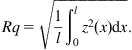 (8.5)
(8.5)The Rq parameter is another popular parameter along with Ra. It is common to see it stated that Rq is always 11 % larger than Ra for a given surface. However, this is only true of a sinusoidal surface, although Rq will always be larger than Ra. The reason for the commonality of Ra and Rq is chiefly historical. The Ra parameter is easier to determine graphically from a recording of the profile and was, therefore, adopted initially before automatic surface texture measuring instruments became generally available. The Rq parameter is used in optical applications where it is more directly related to the optical quality of a surface. Also, Rq is directly related to the total spectral content of a surface.
8.2.7.3 Skewness of the assessed profile, Rsk
Skewness is a measurement of the symmetry of the surface deviations about the mean reference line and is the ratio of the mean cube value of the height values and the cube of Rq within a sampling length,
(8.6)
The Rsk parameter describes the shape of the topography height distribution. For a surface with a random (or Gaussian) height distribution that has symmetrical topography, the skewness is zero. The skewness is derived from the amplitude distribution curve (see Section 8.2.9.5); it is the measure of the profile symmetry about the mean line. This parameter cannot distinguish whether the profile spikes are evenly distributed above or below the mean plane and is strongly influenced by isolated peaks or isolated valleys. Skewness represents the degree of bias, either in the upward or downward direction, of an amplitude distribution curve. A symmetrical profile gives an amplitude distribution curve that is symmetrical about the centre line and an unsymmetrical profile results in a skewed curve. The direction of the skew is dependent on whether the bulk of the material is above the mean line (negative skew) or below the mean line (positive skew). Figure 8.9 shows three profiles and their amplitude distributions curves, with positive, zero and negative skewness. Use of the skewness parameter can distinguish between two surfaces having the same Ra value.

As an example, a porous, sintered or cast iron surface will have a large value of skewness. A characteristic of a good bearing surface is that it should have a negative skew, indicating the presence of comparatively few peaks that could wear away quickly and relatively deep valleys to retain lubricant traces. A surface with a positive skew is likely to have poor lubricant retention because of the lack of deep valleys in which to retain lubricant traces. Surfaces with a positive skewness, such as turned surfaces, have high spikes that protrude above the mean line. The Rsk parameter correlates well with load-carrying ability and porosity.
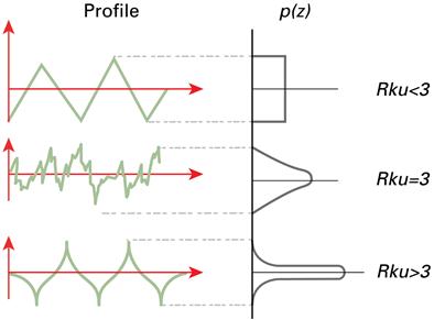
8.2.7.4 Kurtosis of the assessed profile, Rku
The Rku parameter is a measure of the sharpness of the surface height distribution and is the ratio of the mean of the fourth power of the height values and the fourth power of Rq within the sampling length,
(8.7)
The Rku parameter characterises the spread of the height distribution. A surface with a Gaussian height distribution has a kurtosis value of three. Unlike the Rsk parameter, kurtosis can not only detect whether the profile spikes are evenly distributed but also provides a measure of the spikiness of the area. A spiky surface will have a high kurtosis value and a bumpy surface will have a low kurtosis value. Figure 8.10 shows two profiles with low and high values of Rku. This is a useful parameter in predicting component performance with respect to wear and lubrication retention. Note that kurtosis cannot differentiate between a peak and a valley.
8.2.8 Spacing parameters
8.2.8.1 Mean width of the profile elements, RSm
The RSm parameter is the mean value of the profile element widths within a sampling length (Figure 8.11). In other words, this parameter is the average value of the length of the mean line section containing a profile peak and an adjacent valley. This parameter requires height and spacing discrimination. If these values are not specified, then the default height discrimination used is 10 % of Rz. The default spacing discrimination is 1 % of the sampling length and both of these conditions must be met.
8.2.9 Curves and related parameters
The profile parameters described so far have resulted in a single number (often with a unit) that describes some aspect of the surface. Curves and related parameters give much more information about the surface from which, often, functional information can be gained [3]. All curves and related parameters are defined over the evaluation length rather than the sampling length.
8.2.9.1 Material ratio of the profile
The material ratio of the profile is the ratio of the bearing length to the evaluation length. It is represented as a percentage. The bearing length is the sum of the section lengths obtained by cutting the profile with a line (slice level) drawn parallel to the mean line at a given level. The ratio is assumed to be 0 % if the slice level is at the highest peak and 100 % if it is at the deepest valley. Parameter Rmr(c) determines the percentage of each bearing length ratio of a single slice level or 19 slice levels that are drawn at equal intervals within Rt respectively.
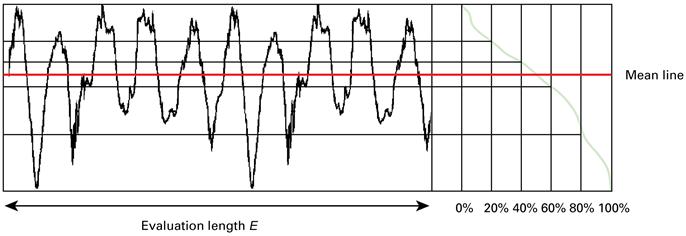
8.2.9.2 Material ratio curve
The material ratio curve (formally known as the Abbot–Firestone or bearing ratio curve) is the curve representing the material ratio of the profile as a function of level. By plotting the bearing ratio at a range of depths in the profile, the way in which the bearing ratio varies with depth can be easily seen and provides a means of distinguishing different shapes present on the profile. The definition of the bearing area fraction is the sum of the lengths of individual plateaux at a particular height, normalised by the total assessment length, and is the parameter designated Rmr (Figure 8.12). Values of Rmr are sometimes specified on drawings; however, such specifications can lead to large ambiguities if the bearing area curve is referred to the highest and lowest points on the profile.
Many mating surfaces requiring tribological functions are usually produced with a sequence of machining operations. Usually, the first operation establishes the general shape of the surface with a relatively coarse finish, and further operations refine this finish to produce the properties required by the design. This sequence of operations will remove the peaks of the original process but the deep valleys will be left untouched. This process leads to a type of surface texture that is referred to as a stratified surface. The height distributions will be negatively skewed, therefore, making it difficult for a single average parameter, such as Ra, to represent the surface effectively for specification and quality-control purposes. A honed surface is a good example of a stratified surface.
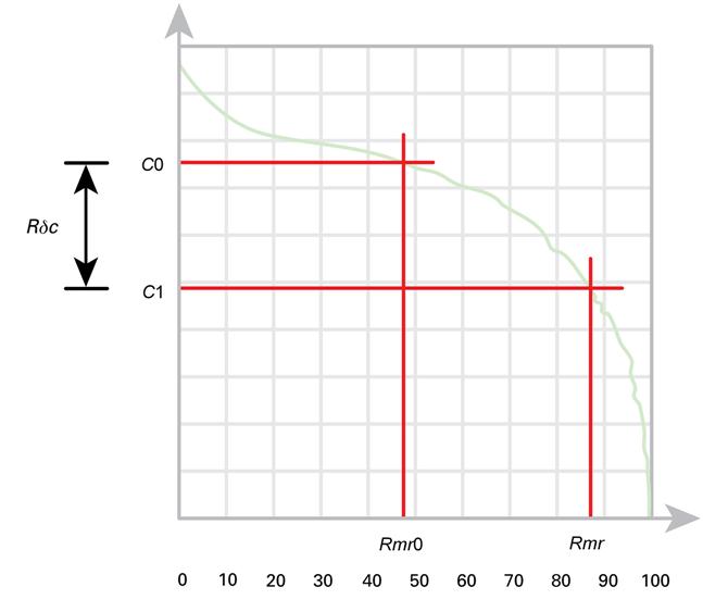
8.2.9.3 Profile section height difference, Rδc
The profile section height difference is the vertical distance between two section levels of given material ratio.
8.2.9.4 Relative material ratio, Rmr
The relative material ratio is the material ratio determined at a profile section level Rδc, and related to a reference, C0, where C1=C0 − Rδc and C0=C(Rmr0). The Rmr parameter refers to the bearing ratio at a specified height (Figure 8.13). A way of specifying the height is to move over a certain percentage (the reference percentage) on the bearing ratio curve and then to move down a certain depth (the slice depth). The bearing ratio at the resulting point is Rmr. The purpose of the reference percentage is to eliminate spurious peaks from consideration – these peaks tend to wear off in early part use. The slice depth then corresponds to an allowable roughness or to a reasonable amount of wear.
8.2.9.5 Profile height amplitude curve
The profile height amplitude curve is defined as the sample probability density function of the ordinate, z(x), within the evaluation length. The amplitude distribution curve is a probability function that gives the probability that a profile of the surface has a certain height, at a certain position. The curve has the characteristic bell shape like many probability distributions (Figure 8.14). The curve tells the user how much of the profile lies at a particular height, in a histogram sense.

The profile height amplitude curve illustrates the relative total lengths over which the profile graph attains any selected range of heights above or below the mean line. This is illustrated in Figure 8.15. The horizontal lengths of the profile included within the narrow band δz at a height z are a, b, c, d and e. By expressing the sum of these lengths as a percentage of the evaluation length, a measure of the relative amount of the profile at a height z can be obtained. Figure 8.15 is termed the amplitude distribution at height z. By plotting density against height, the amplitude density distributed over the whole profile can be seen. This produces the amplitude density distribution curve.

8.2.10 Profile specification standards
There are nine ISO specification standards relating to the measurement and characterisation of surface profile. These standards only cover the use of stylus instruments. The details of the standards are presented elsewhere [10], and their content is briefly described in this section. It should be noted that the current ISO plan for surface texture is that the profile standards will become a subset of the areal standards (see Section 8.3.4). There is also a complete overview of the profile standards taking place in the ISO committee that is responsible for surface texture as part of the geometrical product specification (GPS) system (ISO technical committee 213 working group 16). Whilst the basic standards and details will probably not change significantly, the reader should keep abreast of the latest developments in standards.
ISO 3274 [20] describes a typical stylus instrument and its metrological characteristics. ISO 4287 [11] presents the definitions of the surface profile parameters (i.e. the P, W and R parameters – see Section 8.2.3) and how to calculate the parameters. ISO 4288 [16] describes the various default values and basic rules and procedures for surface texture profile analysis. ISO 16610 part 21 [12] describes the phase correct Gaussian filter that is applied for the various cut-off filters used for surface profile analysis. ISO 12179 [21] presents the methods for calibrating contact stylus instruments for profile measurement, and ISO 5436 part 1 [22] describes the artefacts that are used to calibrate stylus instruments (see Section 6.10.2). ISO 5436 part 2 [23] describes the concepts and use of software measurement standards (see Section 6.15). ISO 1302 [24] presents the rules for the indication of surface texture in technical product documentation such as engineering drawings, specifications, contracts and reports.
Note that there are no specification standards that relate to the measurement of surface profile using optical instruments. However, in many cases, where a profile can be mathematically extracted from an areal optical scan, the profile characterisation and analysis standards can be applied. It is important, however, to understand how the surface data are filtered, especially when trying to compare contact stylus and optical results.
There are no methods specified in ISO standards on how to remove form prior to surface texture analysis (there is work on this subject in ISO technical committee 213 working group 16). The most common form removal filter is the linear least squares method, and this method is applied on some commercial instruments as a default. However, the linear least squares method may be the most appropriate in a large range of cases (especially where low slope angle tilt needs to be removed) but can sometimes lead to significant errors. For example, a linear least squares form removal process will introduce tilt into a sinusoidal surface with few periods within the sampling length. Least squares can also be calculated in two different manners, both leading to potentially different results (see Ref. [25] for details).
ISO 13565 parts 1 [26], 2 [27] and 3 [28] relate to the measurement of surfaces having stratified functional properties. The roughness profile generated using the filter defined in ISO 16610 part 21 (see Section 8.2.3) suffers some undesirable distortions, when the measured surface consists of relatively deep valleys beneath a more finely finished plateau with minimal waviness. This type of surface is very common, for example in cylinder liners for internal combustion engines. ISO 13565 part 1 provides a filtering method of greatly reducing these distortions, thus enabling the parameters defined in ISO 13565 part 2 and part 3 to be used for evaluating stratified surfaces, with minimal influence from these distortions.
In 1970s France, engineers from the school of Arts et Métiers, together with Peugeot and Renault, conceived a graphical method for analysing motifs, adapted to the characterisation of functional surface texture. This method takes the functional requirements of the surface into account and attempts to find relationships between peak and valley locations, and these requirements. The motif method had success in French industry and was incorporated into an international standard in 1996 (ISO 12085 [29]). These motif methods are the basis for the segmentation used in areal feature parameter analysis (see Section 8.3.7).
8.3 Areal surface texture characterisation
There are inherent limitations with 2D surface measurement and characterisation. A fundamental problem is that a 2D profile does not necessarily indicate functional aspects of the surface. With profile measurement and characterisation, it is also often difficult to determine the exact nature of a topographic feature (see Section 6.5). All aspects of areal characterisation, including a range of case studies, can be found elsewhere [9].
8.3.1 Scale-limited surface
Distinct from the 2D profile system, areal surface characterisation does not require three different groups (profile, waviness and roughness) of surface texture parameters as defined in Section 8.2.3. For example, in areal parameters, only Sq is defined for the root mean square parameter rather than the primary surface Pq, waviness Wq and roughness Rq as in the profile case. The meaning of the Sq parameter depends on the type of scale-limited surface used.
Two filters are defined, the S-filter and the L-filter [15,30]. The S-filter is defined as a filter that removes unwanted small-scale lateral components of the measured surface such as measurement noise or functionally irrelevant small features. The L-filter is used to remove unwanted large-scale lateral components of the surface, and the F-operator removes the nominal form (by default using a least squares method [17,31]). The scale at which the filters operate is controlled by the nesting index. The nesting index is an extension of the notion of the original cut-off wavelength and is suitable for all types of filters. For example, for a Gaussian filter, the nesting index is equivalent to the cut-off wavelength. These filters are used in combination to create SF and SL surfaces.
An SF surface (equivalent to a primary surface) results from using an S-filter and an F-operator in combination on a surface, and an SL surface (equivalent to a roughness surface) by using an L-filter on an SF surface. Both an SF surface and an SL surface are called scale-limited surfaces. The scale-limited surface depends on the filters or an operator used, with the scales being controlled by the nesting indices of those filters.
8.3.2 Areal filtering
A Gaussian filter is a good general-purpose filter, and it is the current standardised approach for the separation of the roughness and waviness components from a primary surface (see Section 8.2.3). Both roughness and waviness surfaces can be acquired from a single filtering procedure with minimal phase distortion. The weighting function of an areal filter is the Gaussian function given by
(8.8)
where x, y are the two-dimensional distance from the centre (maximum) of the weighting function, λc is the cut-off wavelength, α is a constant, to provide 50 % transmission characteristic at the cut-off λc, and α is given by
(8.9)
With the separability and symmetry of the Gaussian function, a two-dimensional Gaussian-filtered surface can be obtained by convoluting two one-dimensional Gaussian filters through rows and columns of a measured surface, thus
(8.10)
Figure 8.16 shows a raw measured epitaxial wafer surface (a), its short-scale SL surface (roughness) (b), middle-scale SF surface (waviness) (c) and long-scale form surface (form error surface) (d) by using Gaussian filtering with an automatic correct edged process.

The international standard for the areal Gaussian filter (ISO/DIS 16610-61 [32]) is currently being developed (the areal Gaussian filter has been widely used by almost all instrument manufacturers). It has been easily extrapolated from the linear profile Gaussian filter standard into the areal filter by instrument manufacturers for at least a decade and allows users to separate waviness and roughness in surface measurement.
For surfaces produced using a range of manufacturing methods, the roughness data have differing degrees of precision that contains some very different observations or outliers. In this case, a robust Gaussian filter (based on the maximum likelihood estimation) can be used to suppress the influence of the outliers. The robust Gaussian filter can also be found in most instrument software [15].
It should be noted that the Gaussian filter is not applicable for all functional aspects of a surface, for example in contact phenomena, where the upper envelope of the surface is more relevant. A standardised framework for filters has been established, which gives a mathematical foundation for filtration, together with a toolbox of different filters. Information concerning these filters will soon be published as a series of technical specifications (ISO/TS 16610 series [13]), to allow metrologists to assess the utility of the recommended filters according to applications. The toolbox will contain the following classes of filters:
Linear filters: the mean line filters (M-system) belong to this class and include the Gaussian filter, spline filter and the spline-wavelet filter;
Morphological filters: the envelope filters (E-system) belong to this class and include closing and opening filters using either a disk or a horizontal line;
Robust filters: filters that are robust with respect to specific profile phenomena such as spikes, scratches and steps. These filters include the robust Gaussian filter and the robust spline filter; and
Segmentation filters: filters that partition a profile into portions according to specific rules. The motif approach belongs to this class and has now been put on a firm mathematical basis.
Filtering is a complex subject that will probably warrant a book of its own following the introduction of the ISO/TS 16610 series [13] of specification standards. The user should consider filtering options on a case-by-case basis but the simple rule of thumb is that, if you want to compare two surface measurements, it is important that both sets use the same filtering methods and nesting indexes (or that appropriate corrections are applied). Table 8.2 presents the default nesting indices in ISO 25178 part 3 [31].
Table 8.2
Relationships Between Nesting Index Value, S-filter Nesting Index, Sampling Distance and Ball Radius
| Nesting Index Value (F-operator/L-filter) (mm) | S-filter Nesting Index (μm) | Maximum Sampling Distance (μm) | Maximum Ball Radius (μm) |
| – | – | – | – |
| 0.1 | 1.0 | 0.3 | 0.8 |
| 0.2 | 2.0 | 0.6 | 1.5 |
| 0.25 | 2.5 | 0.8 | 2.0 |
| 0.5 | 5.0 | 1.5 | 4.0 |
| 0.8 | 8.0 | 2.5 | 6.0 |
| 1.0 | 10 | 3.0 | 8.0 |
| 2.0 | 20 | 6.0 | 15 |
| 2.5 | 25 | 8.0 | 20 |
| 5.0 | 50 | 15 | 40 |
| 8.0 | 80 | 25 | 60 |
| 10 | 100 | 30 | 80 |
| 20 | 200 | 60 | 150 |
| 25 | 250 | 80 | 200 |
| 50 | 500 | 150 | 400 |
| 80 | 800 | 250 | 600 |
| 100 | 1000 | 300 | 800 |
| – | – | – | – |

8.3.3 Areal specification standards
In 2002, ISO technical committee 213 formed working group (WG) 16 to address standardisation of areal surface texture measurement methods. WG 16 is developing a number of draft standards encompassing definitions of terms and parameters, calibration methods, file formats and characteristics of instruments. Several of these standards have been published and a number are at various stages in the review and approval process. The plan is that the profile standards will be a subset of the areal standards (with appropriate re-numbering). Hence, the profile standards will be re-published after the areal standards (with some omissions, ambiguities and errors corrected) under a new numbering scheme that is consistent with that of the areal standards. All the areal standards are part of ISO 25178, which will consist of at least the parts given in Table 8.3 (correct at the time of publication), under the general title ‘Geometrical product specification (GPS) – Surface texture: Areal’.
Table 8.3
Current Status of ISO 25178 Areal Specification Standards
| Part | Title | Status | Date |
| 1 | Areal surface texture drawing indications | CD | 2013 [33] |
| 2 | Terms, definitions and surface texture parameters | PS | 2012 [30] |
| 3 | Specification operators | PS | 2012 [31] |
| 4 | Comparison rules | NS | – |
| 5 | Verification operators | NS | – |
| 6 | Classification of methods for measuring surface texture | PS | 2010 [34] |
| 70 | Measurement standards for areal surface texture measurement instruments | FDIS | 2012 [35] |
| 71 | Software measurement standards | PS | 2012 [36] |
| 72 | Software measurement standards – XML file format | CD | 2012 [37] |
| 600 | Nominal characteristics of areal surface topography instruments | WD | 2013 [38] |
| 601 | Nominal characteristics of contact (stylus) instruments | PS | 2010 [39] |
| 602 | Nominal characteristics of non-contact (confocal chromatic probe) instruments | PS | 2010 [40] |
| 603 | Nominal characteristics of non-contact (phase-shifting interferometric microscopy) instruments | PS | 2013 [41] |
| 604 | Nominal characteristics of non-contact (coherence scanning interferometry) instruments | PS | 2013 [42] |
| 605 | Nominal characteristics of non-contact (point autofocus) instruments | FDIS | 2012 [43] |
| 606 | Nominal characteristics of non-contact (variable focus) instruments | CD | 2012 [44] |
| 607 | Nominal characteristics of non-contact (imaging confocal) instruments | WD | 2013 [45] |
| 700 | Calibration of areal surface measuring instruments | WD | 2013 [46] |
| 701 | Calibration and measurement standards for contact (stylus) instruments | PS | 2010 [47] |

Key: WD, working draft; CD, committee draft; NS, not started; DIS, draft international standard; FDIS, final draft international standard; PS, published standards.
Part 1 lists the rules for the indication of surface texture in technical product documentation such as drawings, specifications, contracts and reports. Part 2 lists the definitions of the surface texture parameters (i.e. the field and feature parameters – see Section 8.3.5) and gives details on how to calculate the parameters, including a limited number of case studies. Part 3 describes the various default values, and basic rules and procedures for areal surface topography measurement and characterisation. Whereas the profile analysis standards include a standard on how to filter surface texture data (ISO 16610 part 21 [12]), there are so many filter types available for areal analysis that a new suite of standards is being developed (see Section 8.3.2).
Part 4 on comparison rules and part 5 on verification operators are currently not considered mature enough to be able to produce definitive standards. The part numbers have been reserved for future use when the appropriate research and practical testing on these topics has been established.
Part 6 lists, and briefly describes, the various types of instrument for measuring surface topography. Note that stylus and some of the optical measurement methods listed in part 6 are further described by dedicated parts (the ‘60X series’). However, some measurement techniques do not have an associated 60X equivalent part (e.g. scanning probe or electron beam techniques), but it is expected that these parts will be developed in future standards.
Part 70 describes the artefacts that are used to calibrate areal surface topography measuring instruments and includes the profile calibration artefacts from ISO 5436 part 1 (2000), but with new names (see Section 6.10.3). Part 71 describes the concepts and use of software measurement standards (see Section 6.14) and part 72 an XML file format for the standard data file types described in part 71.
There are four part 60X standards that have been published: part 601 (stylus instruments), part 602 (confocal chromatic probes), part 603 (phase-shifting interferometers) and part 604 (coherence scanning interferometers). At the time of writing, part 605 is at FDIS stage, and 606 and 607 are working drafts. The 60X standards currently contain common terminology, metrological characteristics and a list of parameters that can influence the uncertainties when using the instrument. There are also technical annexes that discuss the theory and operation of the instruments. However, as the 60X series developed, it was realised that there are a large number of sections in the 60X parts that are common to all instruments based on a microscope objective. For example, research has shown that a common set of metrological characteristics can be found that does not differ for each instrument type (see Section 6.12). Therefore, a new standard is under development (part 600), which will cover all the common aspects. Once part 600 is published, the 60X series will be withdrawn and reissued with the common sections removed.
Part 701 is concerned with the calibration of stylus instruments. Part 700, which is still under development, will cover the calibration of instruments and is expected to be common across all instruments. Once part 700 is published, part 701 will be withdrawn.
The American National Standards Institute has also published a comprehensive documentary specification standard, ANSI/ASME B46.1 [48], that includes some areal analyses (mainly fractal based).
8.3.4 Unified coordinate system for surface texture and form
Surface irregularities have traditionally been divided into three groups loosely based on scale [49]: (i) roughness, generated by the material removal mechanism such as tool marks; (ii) waviness, produced by imperfect operation of a machine tool and (iii) errors of form, generated by errors of a machine tool, distortions such as gravity effects, thermal effects, set-up, etc. This grouping gives the impression that surface texture should be part of a coherent scheme with roughness at the smaller scale and errors of form at the larger scale.
The primary definition of surface texture has, until recently, been based on the profile [11]. To ensure consistency of the irregularities in the measured profile, the direction of that profile was specified to be orthogonal to the lay (the direction of the prominent pattern). This direction is not necessarily related to the datum of the surface, whereas errors of form, such as straightness, are always specified parallel to a datum of the surface. Hence, profile surface texture and profile errors of form usually have different coordinate systems and do not form a coherent specification.
This situation has now changed since the draft standardisation of areal surface methods, in which the primary definition of surface texture is changed from one being based on profiles to one based on areal surfaces. This means that there is no consistency requirement for the coordinate system to be related to the lay. Therefore, a unified coordinate system has been established for both surface texture and form measurement [30]. Surface texture is now truly part of a coherent scheme, with surface texture at the smaller scale. The system is part of what is referred to as the GPS.
8.3.5 Areal parameters
There are two main classes of areal parameters:
1. Field parameters – defined from all the points on a scale-limited surface; and
2. Feature parameters – defined from a subset of predefined topological features from the scale-limited surface.
A further class of areal parameters are those based on fractal analysis. Fractal parameters are essentially field parameters but are given their own section in this book as they have certain distinguishing characteristics.
The areal field and feature parameters are described in detail in Refs. [50,51], and a range of case studies illustrating their use are given in Ref. [9]. Further examples of the use of areal parameters can be found in Ref. [52] for the treatment of steel surfaces, Ref. [53] for the characterisation of dental implants, Ref. [54] for the monitoring of milling tool wear and Ref. [55] for the analysis of biofilms.
8.3.6 Field parameters
The field or S- and V-parameter set has been divided into height, spacing, hybrid, functions and related parameters, and one miscellaneous parameter. A great deal of the physical arguments discussed for the profile parameters also apply to their areal equivalents, for example Rsk and Ssk. Therefore, when reading about the areal parameters for the first time, it would be prudent to become acquainted with the description of its profile equivalent (where one exists).
8.3.6.1 Areal height parameters
8.3.6.1.1 Root mean square value of the ordinates, Sq
The Sq parameter is defined as the root mean square value of the surface departures, z(x, y), within the sampling area
(8.11)
 (8.11)
where A is the sampling area, xy. Note that Eq. (8.11) is for a continuous z(x, y) function and the same philosophy applies when converting to a sampled definition as in Section 8.2.7.1.
8.3.6.1.2 Arithmetic mean of the absolute height, Sa
The Sa parameter is the arithmetic mean of the absolute value of the height within a sampling area,
(8.12)
The Sa parameter is the closest relative to the Ra parameter; however, they are fundamentally different and caution must be exercised when they are compared. Areal, or S parameters, use areal filters whereas profile, or R parameters, use profile filters.
8.3.6.1.3 Skewness of topography height distribution, Ssk
Skewness is the ratio of the mean cube value of the height values and the cube of Sq within a sampling area,
(8.13)
The Ssk parameter has very similar features as the Rsk parameter.
8.3.6.1.4 Kurtosis of topography height distribution, Sku
The Sku parameter is the ratio of the mean of the fourth power of the height values and the fourth power of Sq within the sampling area,
(8.14)
The Sku parameter has very similar features as the Rku parameter.
8.3.6.1.5 Maximum surface peak height, Sp
The Sp parameter is defined as the largest peak height value from the mean plane within the sampling area.
8.3.6.1.6 Maximum pit height of the surface, Sv
The Sv parameter is defined as the largest pit or valley depth from the mean plane within the sampling area.
8.3.6.1.7 Maximum height of the surface, Sz
The Sz parameter is defined as the sum of the largest peak height value and largest pit or valley depth value within the sampling area.
8.3.6.2 Areal spacing parameters
The spacing parameters describe the spatial properties of surfaces. These parameters are designed to assess the peak density and texture strength. Spacing parameters are particularly useful in distinguishing between highly textured and random surface structures.
8.3.6.2.1 Auto-correlation length, Sal
For the Sal parameter, it is first necessary to define the auto-correlation function (ACF) as the correlation between a surface and the same surface translated by (tx, ty), given by
(8.15)
The auto-correlation length, Sal, is then defined as the horizontal distance of the ACF(tx, ty) which has the fastest decay to a specified value s, with 0≤s<1. The Sal parameter is given by
(8.16)
For all practical applications involving relatively smooth surfaces, the value for s can be taken as 0.2 [30,50], although other values can be used and will be subject to forthcoming areal specification standards. For an anisotropic surface, Sal is in the direction perpendicular to the surface lay. A large value of Sal denotes that that surface is dominated by low spatial frequency components, while a small value for Sal denotes the opposite case.
The Sal parameter is a quantitative measure of the distance along the surface by which one would find a texture that is statistically different from that at the original location.
8.3.6.2.2 Texture aspect ratio of the surface, Str
The texture aspect ratio, Str, is a parameter used to identify texture strength, that is uniformity of the texture aspect. The Str parameter can be defined as the ratio of the fastest to slowest decay to correlation length, 0.2, of the surface ACF and is given by
(8.17)
In principle, Str has a value between 0 and 1. Larger values, say Str>0.5, indicate uniform texture in all directions, that is for no defined lay. Smaller values, say Str<0.3, indicate an increasingly strong directional structure or lay. It is possible that the slowest decay ACF for some anisotropic surfaces never reaches 0.2 within the sampling area. In this case, Str is invalid.
The Str parameter is useful in determining the presence of degree of lay in any direction. For applications where a surface is produced by multiple processes, Str may be used to detect the presence of underlying surface modifications.
8.3.6.3 Areal hybrid parameters
The hybrid parameters are parameters based on both amplitude and spatial information. They define numerically hybrid topography properties such as the slope of the surface, the curvature of outliers and the interfacial area. Any changes that occur in either amplitude or spacing may have an effect on the hybrid property. The hybrid parameters have particular relevance to contact mechanics, for example the friction and wear between bearing surfaces.
8.3.6.3.1 Root mean square gradient of the scale-limited surface, Sdq
The Sdq parameter is defined as the root mean square of the surface gradient within the definition area,
(8.18)
 (8.18)
The Sdq parameter characterises the slopes on a surface and may be used to differentiate surfaces with similar value of Sa. The Sdq parameter is useful for assessing surfaces in sealing applications and for controlling surface cosmetic appearance.
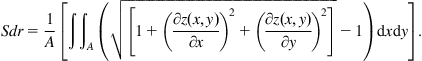
8.3.6.3.2 Developed interfacial area ratio of the scale-limited surface, Sdr
The Sdr parameter is the ratio of the increment of the interfacial area of the scale-limited surface over the definition area and is given by
(8.19)
 (8.19)
The Sdr parameter may further differentiate surfaces of similar amplitudes and average roughness. Typically, Sdr will increase with the spatial complexity of the surface texture independent of changes in Sa. The Sdr parameter is useful in applications involving surface coatings and adhesion and may find relevance when considering surfaces used with lubricants and other fluids. The Sdr parameter may be related to the surface slopes and thus finds application related to how light is scattered from a surface.
8.3.6.4 Functions and related parameters
The functions and related parameters are an areal extension of the profile curves and parameters described in Section 8.2.9.
8.3.6.4.1 Areal material ratio of the scale-limited surface
This is a function representing the areal material ratio of the scale-limited surface as a function of height. The related parameters are calculated by approximating the areal material ratio curve by a set of straight lines. The parameters are derived from three sections of the areal material ratio curve: the peaks above the mean plateau, the plateaux themselves and the valleys between plateaux.
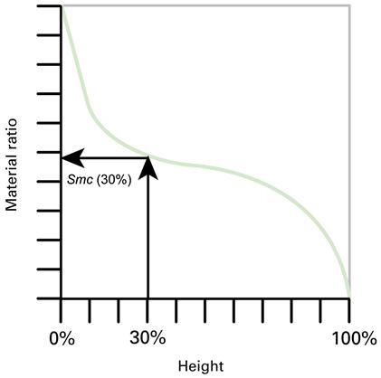
8.3.6.4.2 Areal material ratio of the scale-limited surface, Smc(c)
The areal material ratio is the ratio of the material at a specified height, c, to the evaluation area expressed as a percentage (Figure 8.17). The heights are taken from the reference plane.
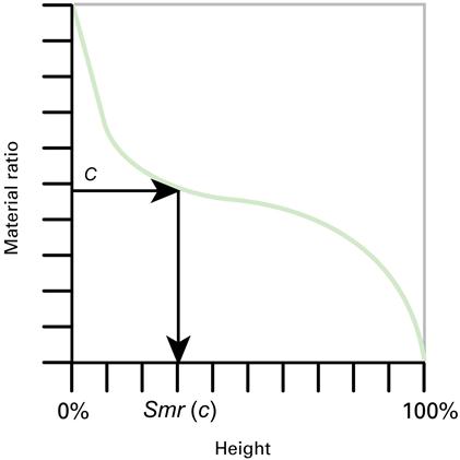
8.3.6.4.3 Inverse areal material ratio of the scale-limited surface, Sdc(mr)
The inverse areal material ratio is the height, c, at which a given areal material ratio, mr, is satisfied, taken from the reference plane (Figure 8.18).
8.3.6.4.4 Areal parameters for stratified functional surfaces of scale-limited surfaces
Parameters (Sk, Spk, Svk, Smr1, Smr2, Svq and Smq) for stratified functional surfaces are defined according to the specification standards for stratified surfaces [27,28].
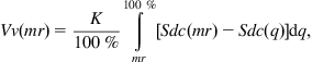
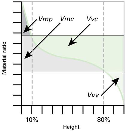
8.3.6.4.5 Void volume, Vv(mr)
The volume of voids per unit area for a given material ratio is calculated from the material ratio curve
(8.20)
 (8.20)
where K is a constant to convert to millimetres per metres squared. The dale volume at p material ratio is given by
(8.21)
and the core void volume (the difference in void volume between p and q material ratio) is given by
(8.22)
where the default values for p (also for Vvv) and q are 10 % and 80 %, respectively [31].
8.3.6.4.6 Material volume, Vm(mr)
The material volume is the volume of material per unit area at a given material ratio calculated from the areal material ratio curve,
(8.23)
 (8.23)
where K is defined as in Eq. (8.20). The peak material volume at p is given by
(8.24)
and the core material volume (or the difference in material volume between p and q material ratio) is given by
(8.25)
where default values for p (also for Vmp) and q are 10 % and 80 %, respectively [31].
Figure 8.19 shows the parts of the material ratio curve that are represented by Vvv, Vvc, Vmp and Vmc.
8.3.6.4.7 Peak extreme height, Sxp
The peak extreme height is the difference in height between p and q material ratio,
(8.26)
where the default values for p and q are 97.5 % and 50 %, respectively [31].
8.3.6.4.8 Gradient density function
The gradient density function is calculated from the scale-limited surface and shows the relative spatial frequencies against the angle of the steepest gradient, α(x, y), and the direction of the steepest gradient, β(x, y), anticlockwise from the x-axis, thus
(8.27)
 (8.27)
and
(8.28)
 (8.28)
8.3.6.5 Miscellaneous parameters
8.3.6.5.1 Texture direction of the scale-limited surface, Std
The texture direction parameter, Std, is the angle, with respect to a specified direction, θ, of the absolute maximum value of the angular power spectrum. The angular power spectrum for an areal surface would be displayed as a 3D plot in which the x- and y-axes represent the various spatial frequencies for a given direction. The amplitude of the angular power spectrum (displayed on the z-axis) represents the amplitude of the sine wave at a particular spatial frequency direction. The angular power spectrum is found by integrating the amplitudes of each component sine wave as a function of angle.
The Std parameter is useful in determining the lay direction of a surface relative to a datum by positioning the part in the measuring instrument in a known orientation. In some applications such as sealing, a subtle change in the surface texture direction may lead to adverse conditions. The Std parameter may also be used to detect the presence of a preliminary surface modification process (e.g. turning), which is to be removed by a subsequent operation (e.g. grinding).
8.3.7 Feature characterisation
Traditional surface texture parameters, that is the profile parameters and the areal field parameters, use a statistical basis to characterise the cloud of measured points. Such parameters, and in particular, profile parameters, were developed primarily to monitor the production process. But, how does a human assess a surface? We do not usually see field parameter values but patterns of features, such as hills and valleys, and the relationships between them [7]. Pattern analysis assesses a surface in the same way. By detecting features and the relationships between them, it can characterise the patterns in surface texture. Parameters that characterise surface features and their relationships are termed feature parameters [56]. Much of the early research work on feature parameters stemmed from work in such areas as machine vision and cartography. A more thorough treatment of feature parameters can be found elsewhere [51].
Feature characterisation does not have specific feature parameters defined, but has instead a toolbox of pattern-recognition techniques that can be used to characterise specified features on a scale-limited surface. The feature characterisation process defined in ISO 25178 part 2 [30] has five stages which are presented in the following sections.
8.3.7.1 Step 1 – Texture feature selection
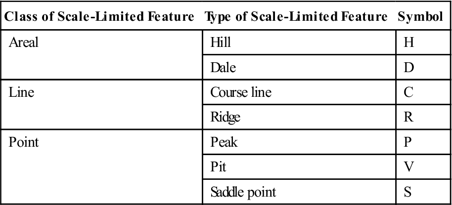
The three main types of surface texture features are areal features, line features and point features (Table 8.4). It is important to select the appropriate type of surface texture feature to describe the function of the surface that is being characterised. The various types of feature will be explained by example in the following sections.
8.3.7.2 Step 2 – Segmentation
Segmentation is used to determine regions of the scale-limited surface that define the scale-limited features. The segmentation process consists of first finding the hills and dales on the scale-limited surface. This usually results in overestimation of the surface and so the smaller, or less significant, segments are pruned out to leave a suitable segmentation of the surface. Some criteria of size that can be used to define a threshold for small segments to prune out are given in Table 8.5.
Table 8.5
Criteria of Size for Segmentation
| Criteria of Size | Symbol | Threshold |
| Local peak/pit height (Wolf pruning) | Wolfprune | % of Sz |
| Volume of hill/dale (at height of connected saddle on change tree) | VolS | Specified volume |
| Area of hill/dale | Area | % of definition area |
| Circumference of hill/dale | Circ | Specified length |
A surface can be divided into regions consisting of hills and regions consisting of dales. Here a hill is defined as an area from which maximum uphill paths lead to one particular peak, and a dale is defined as an area from which maximum downhill paths lead to one particular pit. By definition, the boundaries between hills are course lines and the boundaries between dales are ridge lines. Ridge and course lines are maximum uphill and downhill paths respectively emanating from saddle points and terminating at peaks and pits.
ISO 25178 part 2 [30] defines a dale as consisting of a single dominant pit surrounded by a ring of ridge lines connecting peaks and saddle points, and a hill as consisting of a single dominant peak surrounded by a ring of course lines connecting pits and saddle points. Within a dale or hill there may be other pits or peaks, but they will be insignificant compared to the dominant pit or peak. Figure 8.20 shows a simulated surface and Figure 8.21 shows the corresponding contour representation displaying all the features given in Table 8.4 (a simulated surface has been used for reasons described in Section 8.3.7.2.1).


8.3.7.2.1 Change tree
A useful way to organise the relationships between critical points in hills and dales, and still retain relevant information, is that of the change tree [49,51]. The change tree represents the relationships between contour lines from a surface. The vertical direction on the change tree represents the height. At a given height, all individual contour lines are represented by a point that is part of a line representing that contour line continuously varying with height. Saddle points are represented by the merging of two or more of these lines into one. Peaks and pits are represented by the termination of a line.
Consider filling a dale gradually with water. The point where the water first flows out of the dale is a saddle point. The pit in the dale is connected to this saddle point in the change tree. Continuing to fill the new lake, the next point where the water flows out of the lake is also a saddle point. Again the line on the change tree, representing the contour of the lake shoreline, will be connected to the saddle point in the change tree. This process can be continued and establishes the connection between the pits, saddle points and the change tree. By inverting the surface so that peaks become pits, a similar process will establish the connection between peaks, saddle points and the change tree.
There are three types of change tree:
1. the full change tree (Figure 8.22), which represents the relationships between critical points in the hills and dales;
2. the dale change tree (Figure 8.23), which represents the relationships between pits and saddle points; and
3. the hill change tree (Figure 8.24), which represents the relationship between peaks and saddle points.

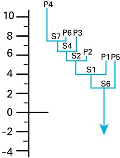

The dale and hill change trees can be calculated from the full change tree.
In practice, change trees can be dominated by very short contour lines due to noise and insignificant features on a surface (this is the reason that a simulated surface was used at the beginning of this section). A mechanism is required to prune the change tree, reducing the noise but retaining significant features. There are many methods for achieving this pruning operation that are too complex to be presented here (see Ref. [57] for a thorough mathematical treatment and Ref. [51] for a more practical description). It is expected that the software packages for feature characterisation will include pruning techniques. One method stipulated in ISO 25178 part 2 [30] is Wolf pruning, and details of this method can be found in Ref. [58].
8.3.7.3 Step 3 – Significant features
It is important to determine the features on a surface that are functionally significant and those that are not. For each particular surface function, there needs to be defined a segmentation function that identifies the significant and insignificant features defined by the segmentation. The set of significant features is then used for characterisation. Methods (segmentation functions) for determining significant features are given in Table 8.6. Once again, it is expected that all these functions will be carried out by the software packages used for feature characterisation. Various research groups are currently developing further methods for determining significant features.
Table 8.6
Methods for Determining Significant Features
| Class of Feature | Segmentation Functions | Symbol | Parameter Units |
| Areal | Feature is significant if not connected to the edge at a given height | Closed | Height is given as material ratio |
| Feature is significant if not connected to the edge at a given height | Open | Height is given as material ratio | |
| Point | A peak is significant if it has one of the top N Wolf peak heights | Top | N is an integer |
| A pit is significant if it has one of the top N Wolf pit heights | Bot | N is an integer | |
| Areal, line, point | All | – |

8.3.7.4 Step 4 – Selection of feature attributes
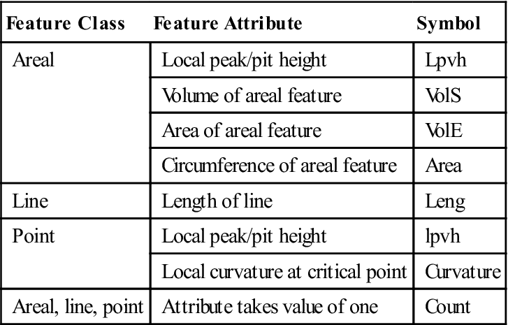
Once the set of significant features have been determined, it is necessary to determine suitable feature attributes for characterisation. Most attributes are a measure of the size of features, for example the length or volume of a feature. Some feature attributes are given in Table 8.7. Various research groups are currently developing further methods for selecting feature attributes and different forms of attribute.
Table 8.7
| Feature Class | Feature Attribute | Symbol |
| Areal | Local peak/pit height | Lpvh |
| Volume of areal feature | VolS | |
| Area of areal feature | VolE | |
| Circumference of areal feature | Area | |
| Line | Length of line | Leng |
| Point | Local peak/pit height | lpvh |
| Local curvature at critical point | Curvature | |
| Areal, line, point | Attribute takes value of one | Count |
8.3.7.5 Step 5 – Quantification of feature attribute statistics
The calculation of a suitable statistic of the attributes of the significant features, a feature parameter, or alternatively a histogram of attribute values, is the final part of feature characterisation. Some attribute statistics are given in Table 8.8. Various research groups are currently developing further methods for quantifying feature attribute statistics.
Table 8.8
| Attribute Statistic | Symbol | Threshold |
| Arithmetic mean of attribute value | Mean | – |
| Maximum attribute value | Max | – |
| Minimum attribute value | Min | – |
| RMS attribute value | RMS | – |
| Percentage above a specified value | Perc | Value of threshold in units of attribute |
| Histogram | Hist | – |
| Sum of attribute values | Sum | – |
| Sum of all the attribute values divided by the definition area | Density | – |
8.3.7.6 Feature parameters
To record the results of feature characterisation, it is necessary to indicate the particular tools that were used in each of the five steps. An example of how to do this that shows the convention is
where FC denotes feature characterisation and the next five symbols, delimited by semicolons, are the symbols from the five tables corresponding to the five steps.
In Sections 8.3.7.6.1–8.3.7.6.9, the default value for X is 5 % [31].
8.3.7.6.1 Density of peaks, Spd
The density of peaks, Spd, is the number of peaks per unit area,
(8.29)
8.3.7.6.2 Arithmetic mean peak curvature, Spc
The Spc parameter is the arithmetic mean of the principle curvatures of peaks with a definition area,
(8.30)
8.3.7.6.3 Ten point height of surface, S10z
The S10z parameter is the average of the heights of the five peaks with largest global peak height added to the average value of the heights of the five pits with largest global pit height, within a definition area,
(8.31)
8.3.7.6.4 Five point peak height, S5p
The S5p parameter is the average of the heights of the five peaks with largest global peak height, within a definition area,
(8.32)
8.3.7.6.5 Five point pit height, S5v
The S5v parameter is the average of the heights of the five pits with largest global pit height, within a definition area,
(8.33)
8.3.7.6.6 Closed dale area, Sda(c)
The Sda(c) parameter is the average area of dales connected to the edge at height c,
(8.34)
8.3.7.6.7 Closed hill area, Sha(c)
The Sha(c) parameter is the average area of hills connected to the edge at height c,
(8.35)
8.3.7.6.8 Closed dale volume, Sdc(c)
The Sdc(c) parameter is the average volume of dales connected to the edge at height c,
(8.36)
8.3.7.6.9 Closed hill volume, Shv(c)
The Shv(c) parameter is the average of hills connected to the edge at height c,
(8.37)
8.4 Fractal methods
Fractal methods have been shown to produce parameters that have a strong ability to discriminate profiles measured from different surfaces and can be related to functional models of interactions with surfaces. There are many ways of analysing fractal profiles [59]. Fractal parameters utilise information about the height and the spacing characteristics of the surface, making them hybrid parameters. Fractal profiles and surfaces usually have the following characteristics:
• they are continuous but nowhere differentiable;
• they are not made up of smooth curves, but rather maybe described as jagged or irregular;
• they have features that repeat over multiple scales;
• they have features that repeat in such a way that they are self-similar with respect to scale over some range of scales;
• they have lengths that tend to increase as the scale of observation decreases;
• they have areas that tend to increase as the scale of observation decreases; and
• they have greater topographic entropy than smooth surfaces.
Many, if not most, measured profiles appear to have the above characteristics over some scale ranges; that is to say that many profiles and surfaces of practical interest may be by their geometric nature more easily described by fractal geometry rather than by the conventional geometry of smooth objects, where the topographic entropy is zero. Topographic entropy increases with the randomness or disorder of the surface and it can be applied to the probability, p, of knowing the height of an intermediate point on a surface given the heights of the adjacent points. Topographic entropy is proportional to the log of 1/p. If the surface is smooth, p is one and the entropy is zero.
To be useful, fractal methods must use multi-scale analyses. This is because measured surfaces demonstrate fractal properties over limited scale ranges, and the fractal properties themselves can change with respect to scale. Multi-scale analysis, that is scale sensitivity, is necessary to be successful in providing the ability to discriminate surfaces that are created by different processes, or that perform differently, and to correlate with topographically related process performance parameters. Correlations and discrimination of the processes are the first kind of performance parameter, and those that relate to the performance are the second kind. The interactions that created the surfaces, and the interactions that are responsible for the performance, tend to occur over limited ranges of scales. Successful discrimination and correlations of the first and second kind is facilitated by being scale specific.
Fractals have some interesting geometric properties. Most interesting is that fractal surfaces have geometric properties that change with scale. Peak and valley radii, inclination of the surface, profile length and surface area, for example, all change with the scale of observation or calculation. This means that a profile does not have a unique length. The length depends on the scale of observation or calculation. This property in particular can be effectively exploited to provide characterisation methods that can be used to model phenomena that depend on roughness and to discriminate surfaces that behave differently or that were created differently. The lack of a unique length is the basis for length-scale analysis.
Fractals are often characterised by a fractional, or fractal, dimension, which is essentially a measure of the complexity of the surface or profile. The fractal dimension for a line will be equal to or greater than one and less than two. The fractal dimension for a surface will be equal to or greater than two and less than three. For mathematical fractal constructs, this characterisation by fractal dimension can be scale insensitive [60]. However, most surfaces of engineering interest are smooth if viewed at a sufficiently large scale, and the fractal dimension can change with respect to scale.
Two approaches have been used to adapt fractal analysis to engineering profiles and surfaces. One approach is to treat the profiles as self-affine, meaning that they have a scaling exponent that varies with scale [61]. The other approach is to divide the scales into regions. For example, most surfaces are rough at fine scales, and smooth at larger scales, and a smooth–rough crossover (SRC) scale can be used to define the boundary between rough (described by fractal geometry) and smooth (described by Euclidean geometry). In the rough region, the fractal dimension can be used to characterise roughness; however, the relative lengths and relative areas at particular scales, which are used to determine the fractal dimension, may be more useful. The SRC is determined as the scale at which the relative lengths or areas exceed a certain threshold. There may be other crossover scales, separating scale regions where different surface creation mechanisms have created geometries with different complexities.
8.4.1 Linear fractal methods
The fractal dimension and the length-scale fractal complexity are determined from the slope of a log-log plot of relative lengths against scale [62]. The relative lengths are the calculated lengths, determined from a series of virtual tiling exercises, divided by the nominal length (Figure 8.25). The nominal length is the straight line length, or the length of the profile used in the length calculation, projected onto the datum. In a virtual tiling exercise, the length of the profile at a certain scale is calculated by stepping along the measured profile with a line segment whose length is that scale. The exercise is repeated in the series by using progressively different lengths and plotting the logarithm of the relative lengths against the logarithm of the corresponding scale for determining that relative length. Linear interpolation is used between measured heights to maintain consistency in the length of the line segments.

The slope of the graph in Figure 8.25 is determined over some appropriate range of scales, where the plot is approximately linear. The scale region is indicated with the slope. Slope multiplied by −1000 is the linear fractal complexity parameter,
(8.38)
One minus the slope of the length-scale plot, whose value is a negative number, is the fractal dimension,
(8.39)
While the slope of the length-scale plot is generally negative or zero, when there are periodic structures on the surface, aliasing can result in small-scale regions with positive slopes. In these cases, local minima in relative lengths can be found at integer multiples of the wavelength of the periodic structures [63]. The finest linear scale in this analysis that has meaning is the sampling interval, and the largest is the length of the measured profile.
Length-scale fractal analysis has found fewer applications than area-scale fractal analysis. Some examples of its use include determining anisotropy for discriminating different kinds of dental microwear [64], discrimination of tool usage, and there is some indication that length-scale fractal analysis may be useful in understanding the skin effect in high-frequency electrical transmissions. The relative lengths as a function of scale have also been used to compare instruments [65,66].
The relative length at a particular scale is related to the inclination on the surface, ϕ, at that scale. Inclinations on a surface vary as a function of scale (Figure 8.26). The relative length parameter is given by
(8.40)
where L is the total nominal length of the profile and pi is the nominal or projected length of the ith segment.

The relative length can give an indication of the amount of the surface that is available for interaction. The relative area, calculated from an areal measurement, however, gives a better indication, because it contains more topographic information.
When the analysed profile is sufficiently long, an SRC can be observed. At the largest scales, the relative lengths will tend towards a minimum weighted average of the reciprocal of the cosine of the average inclination of the analysed profile. If the profile is levelled, this will be one, the minimum relative length. In any case, the slope at the largest scales will be zero so that the fractal dimension will be one, the minimum for a profile. At larger scales, the relative lengths deviate significantly from one and the SRC has been reached. A threshold in relative length can be used to determine the crossover in scale. There may be other crossover scales dividing regions of scale that have different slopes on the relative length-scale plot. This possibility of multiple slopes on the length-scale plot is a characteristic of a scale-sensitive fractal analysis.
8.4.2 Areal fractal analysis
The areal fractal methods are in many ways similar to the linear methods discussed in Section 8.4.1. As with the profile analyses, there are many methods that can be used to estimate the fractal dimension of a rough areal surface. Two areal methods can be found in ISO 25178 part 2 [30]: volume-scale and area-scale methods.
8.4.2.1 Volume-scale analysis
Volume-scale analysis, also known as the variation method, estimates the volume between morphological opening and closing envelopes about a surface. The volume is estimated using nominally square, structuring elements. The size of the structuring elements is varied and the change of volume (Svs) is noted. The logarithm of the volume is plotted against the scale of the elements, that is the length of the sides of the square structuring elements. As the scale increases, so does the volume. The fractal dimension is the slope of the plot, d, plus two. As with the length-scale analysis of engineering surfaces, volume-scale analysis can produce a plot with several slopes in different scale regions with corresponding crossover scales, making this a scale-sensitive type of fractal analysis.
8.4.2.2 Area-scale analysis
Area-scale analysis estimates the area of a rough surface as a function of scale. Area-scale analysis uses repeated virtual tiling exercises of the measured surface with triangles whose area represents the scale of the analysis. For each tiling exercise, the triangles are all the same size. The tiling exercises are repeated with different-sized triangles until the desired range of scales is covered (Figure 8.27).

The maximum range of areal scales that is potentially meaningful in area-scale analysis of a measured surface is found from the finest areal scales, which would be half the square of the sampling interval, to the largest, which would be half of the region measured at the large scales. This is for a measurement that is approximately square with equal sampling intervals in each direction.
Linear interpolation is used between measured heights to maintain consistency in the area of the triangles. The relative area (Srel) is the calculated area divided by the nominal or projected area. Therefore, the minimum relative area is one. As with the relative length, the relative area is an indication of the inclinations on the surface.
The logarithm of the relative area is plotted against the logarithm of the scale to create an area-scale plot. The slope on this graph is related to the area-scale fractal complexity, Safc,
(8.41)
The scale range over which the slope has been determined can also be useful in discriminating surfaces, and in understanding surface texture formation and its influence on surface behaviour. The fractal dimension is given by
(8.42)
The slopes of the area-scale plots used in these calculations are negative. The calculated fractal dimensions are greater than or equal to two and less than three.
The above methods are scale-sensitive fractal analyses, recognising that actual surfaces cannot be well characterised by a single fractal dimension. When the analysed region is sufficiently large, there is an SRC. At the larger scales, the relative areas tend towards the weighted average of the reciprocal of the cosine of the slopes of the unlevelled surface, as shown in Eq. (8.40). The Srel parameter will be one at the large scales if the measured surface is sufficiently large and properly levelled. In any event, the slope of the relative area-scale graph will be generally zero, at sufficiently large scales if a sufficiently large region is analysed. Therefore, the fractal dimension tends towards two, or the Euclidean dimension, at large scales.
Area-scale analysis has a clear physical interpretation for many applications. Many interactions with surfaces are related to the area available to interact and with the inclinations on the surface. The relative area can serve to characterise surfaces in a manner directly related to the functioning for these kinds of interactions. For example, equations for heat, mass and charge exchange contain area terms or density terms implying area. Because the area of a rough surface depends on the scale of observation, or calculation, to use a calculated or measured area for a rough surface in heat, mass or charge exchange calculations, the appropriate scale for the exchange interaction must be known.
Adhesion is an area where area-scale analysis has found application, for example thermal spray coating adhesion [67], bacterial adhesion [68] and carburising [69], which depends on mass exchange. Area-scale analysis also appears useful in electrochemical impedance [70], gloss [71] and scattering [72]. The relative area at a particular scale can be used as a parameter for discrimination testing over a range of scales. This kind of scale-based discrimination has been successful on pharmaceuticals [73], microwear on teeth [63] and ground polyethylene ski bases [74]. Area-scale analysis can also be used to show the effects of filtering by comparing the relative areas of measurements with different filtering at different scales.
Recently, area-scale analysis has also found applications in correlating with oil uptake in fried foods [75,76] which is another example of mass exchange over a surface. Area-scale analysis can also discriminate between the shells of invasive zebra mussels and native clams [77]. Relative area also correlates well with friction of sheet metal of rough dies [78]. Further work points out the importance of scale specificity in finding correlations [79] and suggests that with sufficiently narrow band pass filtering many of the conventional parameters can be indicative of topographic entropy in a specific scale range.
8.5 Comparison of profile and areal characterisation
With the long history and usage of profile parameters, knowledge has been built up and familiarity with profile methods has developed. It will, therefore, often be necessary to compare profile and areal parameters. This section presents some guidance on the fundamental differences between the different classes of parameters and some guidance on their comparison.
The largest difference between profile and areal methods is in the filtration methods used. A profile extracted from an SL surface or an SF surface is not mathematically equivalent to a profile analysed using the methods detailed in the profile standards. The latter uses a profile filter (orthogonal to the lay) and the former an areal filter that can produce very different results even with similar filter types (e.g. Gaussian) and cut-off (or nesting index).
To minimise the difference between profile and areal filtering, the following guidelines should be followed [30,80]:
• the orientation of the rectangular portion of the surface, over which the measurement is made, is aligned with the surface lay;
• a Gaussian filter is used with recommended cut-off value given by the default values in Table 8.1;
• other default values in the profile standards should be used, for example stylus tip radius, sample spacing, etc.; and
• the length in the traverse direction of the rectangular portion of the surface should be five times the cut-off length.
Only those areal parameters that have a direct profile equivalent can be compared, for example the root mean square height parameters Rq and Sq. As a counter example, the texture aspect ratio, Str, has no profile equivalent. Areal surface texture parameters that characterise the extrema of the surface, for example, maximum peak height, Sp, tend to have larger measured values than their equivalent profile parameters since the peaks and valleys on a measured profile nearly always go over the flanks of the peak or valley and not the true extremes.