Operations
This chapter discusses choosing the correct meter type for a specific application. The primary consideration for custody transfer measurement is to minimize flow variations by maintaining better control of the flow rate. This may not always be possible, so meters with appropriate ranges, or multiple meters should be selected. Significant financial risk is at stake in this type of operation, and proper operation is vital.
Different types of meters have uncertainties that change in different ways over the range of flow that they can measure. This must be taken into account when choosing a meter. An estimation of the flow metering performance under given operating conditions can be made with an uncertainty calculation. These are explained in the chapter, and some examples of gas differential meter system uncertainties are discussed. Other fluid flow considerations are also outlined.
Keywords
meter type; measurement uncertainty; custody transfer; flow; operating range; rangeability; flow uncertainty
Operational Considerations
After examining flow and fluid conditions, choosing the correct meter type for a specific application is the next step in achieving minimum measurement uncertainty. However, the meter’s limitations must be recognized along with its positive features in order to make the best selection. Most meters operate with a specified uncertainty within stated flow capacity limits. For custody transfer applications, a meter should not be operated for extended periods of time at or below its stated minimum flow or above its stated maximum capacity.
The primary consideration for custody transfer measurement is to minimize flow variations by maintaining better control of the flow rate. At times, this may not be possible, and the need for a meter with a wide ranging flow capacity will be a further consideration in its selection. If a single meter with the required flow capacity to cover the intended operating range with minimum uncertainty does not exist, the use of multiple meters with some type of meter switching control is required.
For example, consider the fuel supplying a process with three heat exchangers. The range of fuel flows required may be from the pilot load to all three exchangers in full load service. This could require a measurement flow range of over 100 to 1. The metering used could be a combination of a positive displacement meter for the low flows and several turbine or orifice meters for the high flows. Other meter types might also be used. At one time, implementing this type of complex metering system with its meter switching controls could have been a problem, but computers and electronic controllers have simplified the situation, and make such multiple metering solutions more practical. Such a metering system can now be easily managed, and flows can be accurately measured, with the total flow for the whole station being reported as a single measurement.
In addition to the problems of operating meters at the extremes of their flow capacities, the secondary equipment that measures pressure, temperature, differential pressure, density or relative density (specific gravity), and flow composition can also have limitations. Typical uncertainty specifications for these devices are stated as a percent of full scale. Selecting an instrument with the wrong range for the parameter to be measured may introduce greater uncertainty.
If the flowing pressure to be measured is 75 pounds per square inch gauge (psig), and it is measured by an instrument with a 1,000 psig range that has a ±0.5% uncertainty at full scale, then the pressure measurement error could be as high as 5 pounds out of 75 or ±6.7% for linear meters and ±3.3% for differential meters. (The reason for the difference in the two values is that the pressure directly influences the linear meter calculation, but its influence on the differential meter’s calculation is decreased due to the square root extraction.)
The best operating range for a metering system is between 25 and 95% of the maximum capacity of the meters. If operational changes do not exceed the range of the meter, it should be selected to operate near its maximum capacity (Figure 8-1).

Operational Influences on Gas Measurement
Table 8-1 is based on the measurement of natural gas with an orifice meter. The exact magnitude of errors and dollars is not as important as realizing that significant financial risk is at stake and proper operation is vital. A similar study should be performed for any custody transfer application.
Table 8-1
| Flowing Temperature Error | |||
| Temperature, °F | Flow, Mcfd | Loss/Day | Loss/Year |
| 2.0 | 3,837 | ||
| 1.8 | 3,641 | ||
| −0.2 iwc Error | 196 | $784 | $286,160 |
| 25.0 | 13,553 | ||
| 24.8 | 13,499 | ||
| −0.2 iwc Error | 54 | $216 | $78,840 |
| 90.0 | 25,678 | ||
| 89.8 | 25,650 | ||
| −0.2 iwc Error | 28 | $112 | $40,880 |
| Reflects an error in differential pressure measurement of −0.2 in. | |||
| Static Pressure Error | |||
| Pressure, psia | Flow, Mcfd | Loss/Day | Loss/Year |
| (Differential of 2.0″) | |||
| 600.00 | 3,837 | ||
| 598.00 | 3,831 | ||
| −2 psi Error | 6 | $24 | $8,760 |
| (Differential of 25.0″) | |||
| 600.00 | 13,553 | ||
| 598.00 | 13,528 | ||
| −2 psi Error | 25 | $100 | $36,500 |
| (Differential of 90.0″) | |||
| 600.00 | 25,678 | $112 | $40,880 |
| 598.00 | 25,632 | ||
| −2 psi Error | 46 | $184 | $67,160 |
| Reflects an error in pressure measurement of −2 psi for differential meter flow rates. | |||
| Flowing Temperature Error | |||
| Temperature, °F | Flow, Mcfd | Loss/Day | Loss/Year |
| (Differential of 2.0″) | |||
| 62.0 | 3,828 | ||
| 60.0 | 3,837 | ||
| +2°F Error | 9 | $36 | $13,140 |
| (Differential of 25.0″) | |||
| 62.0 | 13,519 | ||
| 60.0 | 13,553 | ||
| +2°F Error | 34 | $136 | $49,640 |
| (Differential of 90.0″) | |||
| 62.0 | 25,615 | ||
| 60.0 | 25,678 | ||
| +2°F Error | 63 | $252 | $91,980 |
| Reflects an error in temperature of +2°F for differential meter flow rates. | |||

Natural gas prices have risen significantly since it was first commercialized, and prices as high as $15 per Mcf have been experienced. Table 8-1 shows the influence of small errors on calculated volumes. Although the examples are based on errors due to instrumentation reading low, similar calculations can be made for instrumentation reading high. The calculations are based on a single 8 inch meter tube using a 4.000 inch bore orifice plate and a gas with a relative density (specific gravity) of 0.580 and 0% carbon dioxide and nitrogen. Volumes are calculated using differential pressures of 2.0, 25, and 90 inches water column (iwc), static pressure of 600 psia, and flowing temperature of 60°F to show the monetary impact of small calibration and/or operating errors. A price of $4/Mcf was used to show revenue errors.
As noted, each meter type has its optimum area of operation for achieving minimum uncertainty, and meters must be matched to the rangeability of the expected flows to be measured. If the flows are steady day in and day out, a meter with a limited rangeability may be all that is needed to handle the application. However, most flow rates in the oil and gas industry change continually. Selecting the metering to accommodate varying flow rates with minimum uncertainty then becomes a major consideration in the design and operation of a meter station. Most meters encounter greater uncertainty in the lower 0 to 10% of their flow capacity. Therefore, if the flow range to be measured includes this area of operation, appropriate designs, using multiple meters, expanded readout systems, and/or characterization of the meters must be employed.
Another way to look at the influence of the flowing conditions on uncertainty is to plot “variation” (error) versus the parameter as in the four charts in Figures 8-2–8-5.


A common misconception is that all meter types maintain the same uncertainty over their entire flow capacity. This tends to be a good assumption for linear meters, but is not true of differential meters. Linear meters normally have an uncertainty that is stated as a percentage of flow or reading, whereas differential meters normally have an uncertainty that is stated as a percentage of full scale or maximum capacity.
For example, a turbine meter has a flow uncertainty expressed as a percentage of flow rate. The uncertainty statements for temperature, pressure (on both linear and differential meters) and differential pressure for differential meters are stated as a percentage of full scale or maximum calibrated span. To summarize this subject, uncertainties in metering are stated in one of two ways: percentage of actual flow rates or reading; or percentage of maximum capacity or full scale.
To make a proper comparison of the “uncertainty” numbers, the statement of each meter’s uncertainty with all operating limitations must be known. These numbers guide an operator in selecting the meter’s optimum capacity range in order to obtain minimum uncertainty.
For a meter with a percentage of flow rate uncertainty statement (such as turbine or ultrasonic), the uncertainty is the same over its entire stated capacity range. The uncertainty of “percentage of maximum capacity” meters can be directly compared to the uncertainty of “percentage of flow rate” meters only at their maximum capacities. Below maximum capacity or full scale, the percentage uncertainty increases as the flow rate decreases for “percentage of maximum capacity” meters, while for “percentage of flow rate” meters uncertainty remains unchanged. Therefore, the two meters’ uncertainties are not directly comparable at lower flow rates.
The significance of flow rate differences on uncertainty is now apparent. When metering systems consist of multiple meters for flow measurement, the uncertainty of all transmitters must be considered to estimate overall system uncertainty. It is very important that each transmitter’s uncertainty be stated in the same terms to make a valid statement of the calculated overall system uncertainty. Likewise, point calibrating a transmitter in a narrow range of operation (such as temperature and pressure) may produce less uncertainty over a limited range than the manufacturer’s stated overall uncertainty.
Most gas metering systems with properly selected, installed, operated, and maintained meters and transmitters should achieve measurement uncertainties under actual operating conditions in the range of ±1%. However, improperly applied meters can misinform a user who does not have a complete knowledge of their operational limitations.
Uncertainty
An estimation of the flow metering performance under given operating conditions can be made with an uncertainty calculation. Many uncertainty calculation procedures are available in the industry standards and flow measurement literature, such as ANSI/ASME MFC-2M, “Measurement Uncertainty for Fluid Flow in Closed Conduits.” The value of an uncertainty calculation is not so much in the absolute value obtained, but rather in the relative comparison of the overall system to the uncertainty of other meters or metering systems, and in exploring the sensitivity of individual components—differential pressure, static pressure, flowing temperature, etc.—in the measurement system.
Such calculations must utilize the particular operating conditions for a specific application in order to be most useful in obtaining minimum measurement uncertainty.
Equation 8.1 shows the calculation of uncertainty for an orifice meter. It is, therefore, representative of differential meters in general and also shows the manner in which the calculation can be made for any meter. The equation for the calculation is divided into two types of error—bias (B) and precision (S)—then these are combined as the square root of the sum of the squares.
(8.1)
This equation will calculate the uncertainty of a flow measurement, assuming the variables are measured over a long time period. The uncertainty represents deviation from the true value for 95 percent of the time. The value of the calculation will depend on the accuracy of the values used for the bias and precision errors. Individual component uncertainties are weighted, based on the manner in which they influence the flow calculation. In the simplified orifice equation:
(8.2)
where:
Q=rate of flow in appropriate units;
K=a coefficient based on the mechanical installation and other flow variables;
d=orifice bore diameter in appropriate units;
dP=differential pressure in appropriate units;
P=absolute static pressure in appropriate units.
The values are either direct multipliers, squared, inverse, or square root values. The weighting values have a sensitivity factor of either 1 or −1 for direct multiplied variables, a sensitivity factor of 2 for squared value, and a sensitivity factor of 1/2 for square root value multiplied by component uncertainties. Thus, in the simplified orifice meter uncertainty Equation 8.2, the uncertainty in Κ is multiplied by 1, the uncertainty in d is multiplied by 2, and the uncertainty in dp and Ρ are multiplied by 1/2. Thus, the uncertainty in orifice meter flow rate would be:
(8.3)
The values used for the precision uncertainties in the equation may be obtained from the manufacturers’ specifications for the respective pieces of equipment, provided that the values are adjusted to reflect operating conditions. The bias uncertainties must be determined by testing.
Examples of Gas Differential Meter System Uncertainties
Since there are many combinations of equipment, operating conditions and calculation methods in existence for orifice metering, it is impossible to establish a single base line uncertainty relationship. The most practical approach is to provide uncertainty ranges for the most typical differential metering combinations. The following orifice metering system combinations have been selected as examples of system uncertainty estimations (Table 8-2):
• Chart metering system (upper range) operating under AGA Report No. 3 (1985) with differential pressure averaging 10 inches of water column (iwc), single static pressure and temperature, and standard calibration equipment accuracy.
• Chart metering system (lower range) operating under AGA Report No. 3 (1990 to 1992) with differential pressure averaging 50 iwc and premium calibration equipment accuracy.
• Electronic metering system (upper range) operating under AGA Report No. 3 (1985) with differential pressure averaging 10 iwc, single static pressure and temperature, and standard calibration equipment accuracy.
• Electronic metering system (lower range) operating under AGA Report No. 3 (1990 to 1992) with differential pressure averaging 50 iwc and premium calibration equipment accuracy.
• For the purpose of establishing the orifice meter measurement uncertainty ranges, the following conditions are assumed:
• The variables Ρf, Tf, and Gr are functioning at 70% of full scale.
• Ambient temperature influences are maintained at ±15°F through monthly calibrations.
• The differential pressure variable, dp, is maintained between 10 and 95% of full scale.
• All meter runs are of the same size with the same bore orifice plates.
Table 8-2
Orifice Meter System Uncertainty Examples
| Element | Chart System Element % Accuracy Upper Range | Chart System Element % Accuracy Lower Range | Electronic System Element % Accuracy Upper Range | Electronic System Element % Accuracy Lower Range |
| Cd | 0.600 | 0.440 | 0.600 | 0.440 |
| Y | 0.030 | 0.010 | 0.030 | 0.010 |
| d | 0.050 | 0.020 | 0.050 | 0.020 |
| D | 0.250 | 0.010 | 0.250 | 0.010 |
| dp | 0.500 | 0.500 | 0.150 | 0.150 |
| Pf | 1.000 | 1.000 | 0.250 | 0.200 |
| Tf | 1.000 | 1.000 | 0.250 | 0.100 |
| Fpv | 0.100 | 0.100 | 0.100 | 0.100 |
| Gr | 0.500 | 0.100 | 0.500 | 0.100 |
| dpc | 0.100 | 0.050 | 0.100 | 0.050 |
| Ρfc | 0.100 | 0.050 | 0.100 | 0.050 |
| Tfc | 0.067 | 0.067 | 0.067 | 0.067 |
| Grc | 0.167 | 0.167 | 0.167 | 0.167 |
| Single Meter Run Calculated % Uncertainty | Single Meter Run Calculated % Uncertainty | Single Meter Run Calculated % Uncertainty | Single Meter Run Calculated % Uncertainty | |
| 2.85 | 1.20 | 1.19 | 0.60 |

Where:
Orifice meter coefficient of discharge, Cd
Expansion factor, Y
Orifice bore diameter, d
Meter tube inside diameter, D
Differential pressure, dp
Static pressure, Pf
Flowing temperature, Tf
Gas compressibility factor, Zf & Zb (Fpv)
Gas relative density, Gr
Differential pressure calibrator, dpc
Static pressure calibrator, Pfc
Flowing temperature calibrator, Tfc
Gas relative density calibrator, Grc
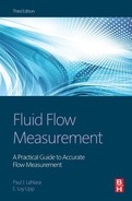
Figures 8-6 and 8-7 provide the results of the chart and electronic system multiple meter tube orifice meter uncertainty calculations.

Example of Gas Linear Meter System Uncertainties
Since there are numerous combinations of equipment, operating conditions, and calculation methods in existence for linear metering, it is impossible to establish a single uncertainty relationship. The most practical approach is to provide uncertainty ranges for the most typical linear metering combinations.
The following have been selected as the most typical linear metering combinations (Table 8-3):
• Chart metering system (upper range) with linear meter operating at less than 1% of capacity, single static pressure and temperature, and standard calibration equipment accuracy.
• Chart metering system (lower range) with linear meter operating from 10 to 100% of capacity and premium calibration equipment accuracy.
• Electronic metering system (upper range) with linear meter operating at less than 1% of capacity, single static pressure and temperature, and standard calibration equipment accuracy.
• Electronic metering system (lower range) with linear meter operating from 10 to 100% of capacity and premium calibration equipment accuracy.
Table 8-3
Linear Meter Element Uncertainty Examples
| Element | Chart System Element % Accuracy Upper Range | Chart System Element % Accuracy Lower Range | Electronic System Element % Accuracy Upper Range | Electronic System Element % Accuracy Lower Range |
| PML | 2.000 | 0.500 | 2.000 | 0.250 |
| Pf | 1.000 | 0.500 | 0.250 | 0.200 |
| Tf | 1.000 | 0.500 | 0.250 | 0.100 |
| Zf | 0.250 | 0.100 | 0.250 | 0.100 |
| Gr | 0.500 | 0.100 | 0.500 | 0.100 |
| PMfc | 0.500 | 0.300 | 0.500 | 0.300 |
| Pfc | 0.100 | 0.050 | 0.100 | 0.050 |
| Tfc | 0.067 | 0.067 | 0.067 | 0.067 |
| Grc | 0.167 | 0.167 | 0.167 | 0.167 |
| Single Meter Run Calculated % Uncertainty | Single Meter Run Calculated % Uncertainty | Single Meter Run Calculated % Uncertainty | Single Meter Run Calculated % Uncertainty | |
| 3.24 | 1.36 | 2.58 | 0.73 |

Where:
Positive meter linearity, PML
Static pressure, Pf
Flowing temperature, Tf
Gas compressibility factor, Zf & Zb
Gas relative density, Gr
Positive meter flow calibrator, PMfc
Static pressure calibrator, Pfc
Flowing temperature calibrator, Tfc
Gas relative density calibrator, Grc
For the purpose of establishing the linear meter measurement uncertainty ranges, the following conditions are assumed:
• The variables Pf, Tf, and Gr are functioning at 70% of full scale.
Ambient temperature influences are maintained at ±15°F through monthly calibrations.
• All meter runs are of the same size with the same size meters.
Figures 8-8 and 8-9 provide the results of the chart and electronic system multiple meter tube linear meter uncertainty calculations. These are “lost and unaccounted for” control charts.


The foregoing is a somewhat detailed description of the influence of only one of the factors in determining uncertainty from the equation. Many other values should be similarly examined.
Calculation of the uncertainty associated with the variables in the flow equation is not the only concern for a complete uncertainty determination. Allowance must be made for human interpretation influence, chart integration or computer influence, installation influence, and fluid characteristic influence. Most of these influences are minimized, provided industry standard requirements are met and properly trained personnel are responsible for the operation and maintenance of the station. Since these effects cannot be quantified, they are minimized by recognizing their potential existence and properly controlling the meter station design, operation, and maintenance. Without proper attention to the total problems, a simple calculation of the equation variables may mislead a user into believing that measurement is better than it actually is.
If maintenance is neglected and the measurement experiences abnormal influences, such as contaminant deposits that change its flow characteristics, then the calculation is meaningless until those abnormal influences are removed.
Operating Influences on Liquids
The liquid metering systems most commonly used in the oil industry are turbine metering, positive displacement (PD) metering, and tank gauging. Additionally, the use of ultrasonic and Coriolis meters is growing rapidly. Turbine meters and PD meters measure the flowing stream dynamically, while tank gauging is a static measurement. Both types of metering are covered extensively in the API Manual of Petroleum Measurement Standards (MPMS), and measurement systems must be operated in accordance with their recommendation in order to obtain measurement with a minimum uncertainty. Physical properties and operational constraints will determine a specific system for each application.
Minimizing the uncertainty of a liquid metering system depends on knowing the system’s limitations and operating within them. Some system limitations include:
• Flow rate within calibrated range;
• Viscosities higher or lower than that experienced during calibrations;
For turbine and PD meters, a general review should include:
• Is the station actually operating within the design flow range?
• Is the system designed to take into account all of the physical properties, such as temperature, pressure, density or relative density, and to be compatible with any corrosive characteristic of the fluid to be measured?
• Is the meter protected from excessive operating conditions, such as liquid surges, entrained gases (flashing), pulsations, and excessive pressure, and are the protective devices such as pressure relief, surge tanks, and vapor removal equipment installed and operating properly?
• Is the flowing environment clean (especially important for turbine meters)?
• If the liquid has a high vapor pressure, is back pressure monitored and controlled?
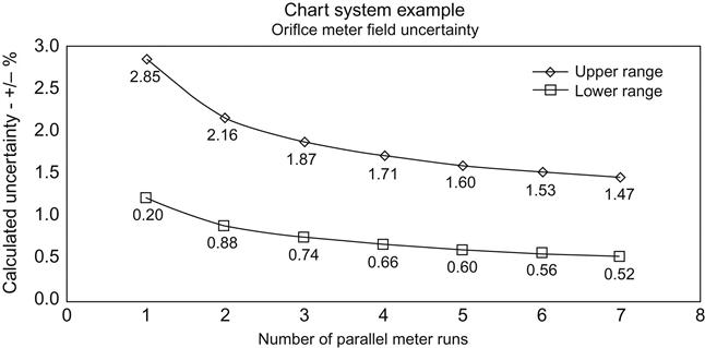
The influence of these conditions can be identified and tracked by the use of an operating system control chart such as shown in Figure 8-10.

The value of good measurement should be obvious to the readers of this book. To obtain this quality of measurement there are two main areas affecting meter operation: system parameters and meter parameters.
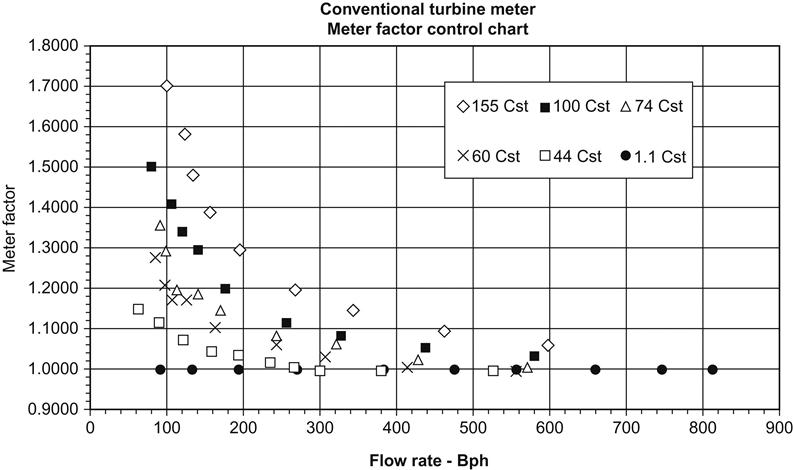
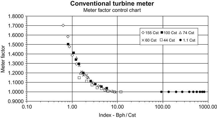
System parameters should include fluid viscosity. Both turbine meters’ and positive displacement meters’ performance can be affected by liquid viscosity. A PD meter is more linear than a turbine meter at higher viscosities. As viscosities increase, a turbine meter’s meter factor can become significantly non-linear. On the other hand, PD meters tend to be less sensitive to viscosity variations and more concerned with slippage and pressure drop. At lower flow rates, a PD meter factor curve can be affected as viscosity drops due to increased slippage. As viscosities go up, pressure drop increases and meter wear is increased. If the liquid viscosity changes widely, meter performance will be affected by the deviations as shown in the previous charts. Examples of the influence of varying viscosity on the performance of PD meters and two types, conventional and helical, of turbines meters are shown in Figures 8-10a, 8-10c, and 8-10e. In addition, Figures 8-10b, 8-10d, and 8-10f show how the performance of these meters can be improved by characterization using the information from meter factor control charts.


When searching for sources of increased meter uncertainty (particularly in liquid applications), it is necessary to investigate viscosity changes and correlate them with meter performance.
Other Fluid Flow Considerations
Liquid flow rate can affect meter uncertainty. When examining a metering system, it is necessary not only to examine the total volumes measured, but also to know how any variations in meter flow rate influence the uncertainty in the total volume delivered.
The influence of temperature fluctuations must also be considered. In addition to affecting viscosity, liquid temperature can also change the mechanical clearances in PD meters and the measuring chamber volumes; changes in mechanical clearances may necessitate the use of extra clearance rotors. Additional mechanical clearance allows for different thermal expansions of the rotor and housing, and prevents meter lockup.
When proving meters, temperature equilibrium should be maintained throughout the meter and prover system. Where extremes of ambient or flowing fluid temperatures are experienced, it may be necessary to insulate the system to obtain stabilization. Temperature stabilization may require some run time before proving is attempted, since unstable temperatures will usually result in erratic provings.
System flow rate must be known so that the meter range can be checked. Rating a meter so it operates in its mid-range (10 to 95% of the meter’s stated range) will usually result in minimum uncertainty.
The nature of the liquid to be metered is critical to the selection of meter type. Metal in contact with flowing fluids must be compatible with the characteristics of the liquid to be measured. The liquid should be free of entrained air and abrasive solids. To eliminate air, an air eliminator can be installed upstream of the meter. It should be tested to insure proper operation. Likewise, a separator with properly sized mesh should be installed to remove the solids, and this should be checked periodically. Air that has not been removed will be measured as liquid. A slug of air followed by liquid into a turbine meter can destroy the turbine rotor and/or its bearings.
Meter Parameters
The most important parameter in a meter’s operation is its proving results. For both PD and turbine meters, changes in the meter factor curve outside of acceptable tolerances are an indication that an effective change is taking place, which may signal the need to disassemble the meter to repair any damage. The meter provings should be summarized in a meter factor control chart that can be monitored to identify changes in meter performance.
In general, a turbine meter’s factor begins to become non-linear at flow rates equal to, or below, 5% of the meter’s maximum capacity. This is a point where bearing friction can become significant. With higher viscosities, the point of deviation may be as high as 35% of maximum capacity. Turbine meters are normally monitored electronically, so any losses due to readout should be insignificant. Once a base meter factor curve has been established for a meter, changes outside established bounds will indicate cleaning or replacement is needed.
Rangeability
PD meters have a usable flow range of between 50:1 and 100:1. The turbine meter has about a 10:1 range with low viscosity liquids or with viscosity characterization (indexing). A turbine meter’s usable range decreases at higher viscosities without indexing and with decreasing relative density (relative density of 0.55 or less).
Repeatability
The repeatability of a properly applied PD meter should be in the range of ±0.05% or better with the same flowing parameters. Turbine repeatability should be ±0.02% or better when the meter is operating properly. Unless a turbine meter is mechanically impaired, it will maintain its repeatability even when the meter becomes non-linear.
Pressure Drop
As previously indicated, pressure drop is affected by many factors including:
Any significant change in pressure drop will signal that inspection and/or repairs should be scheduled as soon as possible. Typically, the pressure drop on a turbine meter is about 4 psi at maximum flow (6 psi at 130% flow) on water and is a function of each meter’s internal design. At higher viscosities, the pressure drop will be larger. Pressure drop does not pose the same potential problem for a turbine meter that it does for a PD meter.
Output Signal
The output signal may be obtained through mechanical gearing systems or via an electronic pickup that produces a pulse signal. Turbine meters normally use an electronic readout.
Summary
There are a number of system and meter parameters that affect meter performance. By being aware of these concerns, a user can obtain the optimum performance from a meter that is maintained and operated properly. Installing a meter with excellent performance potential without providing for its proper operation and maintenance represents waste and incompetence.
Tank Gauging
In tank gauging, the most important parameters to measure correctly are:
Proper level measurement, correct tank dimensions, and proper temperature are all critical. Since temperature stratification may take place in a tank, getting a representative average temperature may be difficult. Several procedures are specified and must be used in accordance with the appropriate types of vessel, such as storage tank, tank cars, and trucks. Another concern is wall retention, i.e., the amount of the fluid that may adhere to the wall within a tank.
Tank strappings on all vessels should be up to date. A tank should have a solid foundation under its floor, and the walls should not be flexible. The walls should be clean and not encrusted.
The general rule of thumb is that the best uncertainty (0.15%) obtained when using tank gauging occurs when the entire volume of a completely full tank is withdrawn. When a very small amount (in the order of 4%) is withdrawn from a 100% full tank, the uncertainty suffers and can be in the order of 3%. Again when the entire volume of a 15% full tank is withdrawn the uncertainty will suffer and can be as great as 0.66%.
It Pays to Protect Investment
Operating flow measurement problems are solved by dedicating people, time, and money to ensuring that the meters and equipment are operating properly. Delivery variances are thus minimized and terminals and pipelines inventories are controlled. To aid in finding problems in the case of an imbalance, documentation should be maintained that shows that the calculations, procedures, and equipment operation have been performed in accordance with the industry standards and contract requirements.
Some flows are difficult to measure accurately with any meter. Once these are identified, the operator must accept greater uncertainty in the measurement, or should improve the flowing conditions to allow more accurate measurement. It is imperative that any meter’s limitations be recognized and fitted to the operating requirements of the flows to be measured. The performance potential of a meter is of no value if it is not installed, operated, and maintained in such a manner that its potential can be realized.