CHAPTER 12
Decision Trees
Chapter 10 and Chapter 11 described tree algorithms in general and balanced trees in particular. They explained algorithms that you can use to build and maintain trees, but they didn't describe any algorithms that use trees to solve a particular problem.
This chapter describes decision trees, which you can use to model situations where you can solve a problem by making a series of decisions. Each branch in the tree represents a single choice. A leaf node represents a complete set of decisions that produces a final solution. The goal is to find the best possible set of choices or the best leaf node in the tree.
For example, in the partition problem, you want to divide a set of objects of various weights into two groups that have the same total weight. You could model this problem with a binary tree, where the left branch at level K of the tree corresponds to including the Kth object in the first pile and the right branch corresponds to including the Kth object in the second pile. A complete path through the tree corresponds to a complete assignment of objects to the two piles. The goal is to find a path that gives the most even distribution of weight.
Decision trees are extremely useful and can model all sorts of situations where you can use a series of steps to produce a solution. Unfortunately, decision trees are often truly enormous. For example, the binary tree described in the preceding paragraph representing the division of N objects into two piles has ![]() leaf nodes, so searching the entire tree may be impossible. For example, a tree representing the division of 50 objects has approximately
leaf nodes, so searching the entire tree may be impossible. For example, a tree representing the division of 50 objects has approximately ![]() leaf nodes. Even if you could examine 1 million of those nodes per second, it would take more than 2,100 years to examine every node.
leaf nodes. Even if you could examine 1 million of those nodes per second, it would take more than 2,100 years to examine every node.
This chapter describes some different kinds of decision trees. It explains techniques that you can use to search these trees efficiently so that you can find solutions to larger problems than you could find by using a brute-force approach. It also explains heuristic methods that you can use to find approximate solutions to some problems when searching a tree completely isn't feasible.
The following section starts the discussion of decision tree search algorithms by covering a very specific kind of search: game tree searches.
Searching Game Trees
You can model games such as chess, checkers, Go, and tic-tac-toe (naughts and crosses) with a game tree where each branch represents a move by one of the players. If at some point in the game a player has 10 possible moves, then the tree at that point has 10 possible branches. A complete path through the tree corresponds to a complete game.
Like all decision trees, game trees grow extremely quickly. For example, suppose that a chess game lasts 40 moves (each player moves 20 times) and has an average of about 30 possible moves per turn. In that case, the total number of paths through the game tree is roughly ![]() . Exhaustively searching such a tree with a computer that could examine 1 billion possible paths per second would take roughly
. Exhaustively searching such a tree with a computer that could examine 1 billion possible paths per second would take roughly ![]() years. (See
years. (See https://en.wikipedia.org/wiki/Shannon_number for a discussion of the Shannon number, an estimate of the complexity of chess.)
Tic-tac-toe is a more tractable problem, although the game tree is still huge. In the first move, the X player initially has nine choices. In the second move, player O has eight choices because one square is already taken by X. At each move, the current player has one fewer choice than the other player had in the previous move, so a total of ![]() paths are possible through the game tree.
paths are possible through the game tree.
Some of those paths are illegal. For example, if X takes the top three squares in the first moves, the game is over, so any paths through the tree that begin with X taking those squares don't go all the way to the ninth level of the tree.
If you remove all of the paths that end early, the game tree still contains roughly a quarter-million leaf nodes, so the tree is still fairly large.
The following sections describe algorithmic techniques that you can use to search a tic-tac-toe game tree. The discussion uses tic-tac-toe because that problem is reasonably small, but the same techniques apply to any similar game, such as chess, checkers, or Go.
Minimax
To decide whether one move is preferable to another during a game, you need to decide what value the different board positions have. For example, if you can place an X in a particular square in a tic-tac-toe game and doing so lets you win, then that board position has a high value. Conversely, if placing an X in a different position will allow O to win later, then that board position has a low value.
Other games such as chess use different board position values that can depend on many factors, such as whether you win, whether your opponent wins, whether your pieces occupy certain parts of the board, and whether your pieces can threaten certain positions. In tic-tac-toe, you can define four board values.
- 4: The board position will end in a win for this player.
- 3: It's unclear whether the current board position will result in a win, loss, or draw.
- 2: The board position will end in a draw.
- 1: The board position will end in a loss for this player.
Figure 12.1 shows board positions demonstrating each of these values. In the upper-left board position, X will win in the next move. The board position in the upper right gives a loss to X, because O will win no matter where X goes in the next turn. The lower-left board position is uncertain, assuming that you can search only a few levels into the game tree. Finally, the board position in the lower right will end in a draw no matter where X and O move on their final moves.

Figure 12.1: To pick a move, the program must assign values to board positions.
There's an obvious relationship among these values. If player 1 wins, then player 2 loses. If a game ends in a draw for player 1, it also ends in a draw for player 2. If the board value is unknown for player 1, then it's also unclear for player 2.
For complicated games, the outcome of a particular board position is often uncertain because the program cannot search the game tree thoroughly enough to examine all of the possible outcomes. In cases such as those, the program must assign approximate values to different positions so that the program can pick the best one.
On a reasonably fast computer, a tic-tac-toe program can search the entire game tree, so the value 3 isn't really necessary. It is included here so that you can see how to handle more complicated games. (You can get the same effect in a tic-tac-toe program by not allowing the program to search more than a few levels through the game tree.)
Minimax is a game tree search strategy in which, at each move, you try to minimize the maximum value your opponent can achieve. For example, if you can make two moves, the first giving your opponent a win and the second giving your opponent a loss, you should take the second move.
The following pseudocode shows the minimax algorithm at a high level:
// Find the best move for player1.Minimax(Board: board_position, Move: best_move, Value: best_value,Player: player1, Player: player2, Integer: depth, Integer: max_depth)// See if we have exceeded our allowed depth of recursion.If (depth > max_depth) Then// We have exceeded the maximum allowed depth of recursion.// The outcome for this board position is unknown.best_value = UnknownReturnEnd If// Find the move that gives player2 the lowest value.Value: lowest_value = InfinityMove: lowest_moveFor Each <possible test move><Update board_position to make the test move>// Evaluate this board position.If <this is a win, loss, or draw> Then<Set lowest_value and lowest_move appropriately>Else// Recursively try other future moves.Value: test_valueMove: test_moveMinimax(board_position, test_move, test_value,player2, player1, depth, max_depth)// See if we found a worse move for player2.If (test_value < lowest_value) Then// This is an improvement. Save it.lowest_value = test_valuelowest_move = test_moveEnd IfEnd If<Restore board_position to unmake the test move>Next <possible test move>// Save the best move.best_move = lowest_move// Convert board values for player2 into values for player 1.If (lowest_value == Win)best_value = LossElse If (lowest_value == Loss)best_value = WinElse…End IfEnd Minimax
The algorithm starts by checking its depth of recursion. If it has exceeded its maximum allowed depth of recursion, the algorithm cannot determine the game's eventual outcome from this board position, so it sets best_value to Unknown and returns.
To find the best move for player1, the algorithm must find the move that gives player2 the worst board value. The algorithm creates variables to keep track of the lowest board value found so far for player2. It sets lowest_value equal to Infinity so that any board value it finds replaces that initial value.
Next the algorithm loops through all the moves that player1 could make. The Minimax algorithm makes a move and then recursively calls itself to find the best move player2 could make after player1 makes that test move.
After the recursive call returns, the algorithm compares the best result player2 could obtain with the value saved in lowest_value. If the test value is lower, the algorithm updates lowest_value and lowest_move, so it knows that this move is preferable (to player1).
After it finishes examining all the possible test moves, the algorithm knows which move player1 should make to give player2 the worst possible board position. It saves that move and then converts the value of the board for player2 into the value for player1. For example, if the best board position makes player2 lose, then it makes player1 win and vice versa.
In cases where player2 doesn't win or lose, it's a little less clear how to convert from a player2 value to a player1 value. For tic-tac-toe, the Unknown and Draw values are the same for both players. For example, if a board position gives player2 a draw, it gives player1 a draw as well.
For a more complicated game such as chess, a board position's value might be a number between –100 and +100, where +100 represents a win and –100 represents a loss. In that case, player2's value for a board position might simply be the negative of player1's value for the same board position.
One side effect of a simple minimax strategy that can sometimes be a problem is that the program considers all solutions that have the same board value equally desirable. To see why that can be a problem, suppose that a game is close enough to the end for the program to realize that it will lose no matter what it does. In that case, it selects the first move it considers while searching the game tree, because all moves give the same result. The result may seem random or even foolish. For example, the program might pick a move that gives its opponent a win in the next move when a different move might have delayed the inevitable for two or three more moves. In contrast, a human would probably pick a move that made the game last longer, hoping the opponent will make a mistake or won't realize that the game is as good as over. Alternatively, a human might concede instead of delaying the inevitable or making seemingly-random moves.
Conversely, the program might find a way to win in six moves and pick that over another strategy that would win in only two moves. If the computer finds the six-move win first, it won't switch later to the two-move win because that doesn't improve the outcome.
You can address these problems by favoring longer sequences of moves that lead to losses or ties and shorter sequences of moves that lead to wins.
A simple minimax strategy is enough for a winning tic-tac-toe game, but for more complicated games, a program cannot search the entire game tree. The following sections describe some strategies that you can use to search larger game trees.
Initial Moves and Responses
One way to reduce the size of the game tree is to store precomputed initial moves and responses. If you search the game tree ahead of time to find the best possible initial move, then you can simply have the program make that move if it has the first turn. Instead of spending a noticeable amount of time searching for a first move, the program can move instantly.
The user moves next, so the computer doesn't need to move again until two moves have been made. The size of the game tree at that point depends on the particular moves made, but the tree will be much smaller than the original game tree. For example, the entire tic-tac-toe game tree contains 255,168 possible games. If X picks the upper-left square and O picks the upper-middle square, the remaining game tree contains only 3,668 possible games. That may still be too many to enumerate by hand, but it's small enough for a computer to search.
If the user moves first, the game tree also shrinks dramatically. If the user picks the upper-left square for the first move, the remaining game tree contains only 27,732 possible games. This is a lot more than the number of games after the second move, but it's still a lot smaller than the entire game tree. With one additional change, you can make that number even smaller.
X has only nine choices for a first move. If you precalculate all of the best responses to those first moves, you can make the program simply look up the appropriate response. Instead of searching a game tree containing 27,732 possible games, the program only needs to look up one of nine possible responses.
The user then moves again, so the program doesn't need to search the game tree until three moves have been made—one by the user, one a precalculated response, and another by the user. At that point, the game tree is much smaller. For example, if X takes the upper-left square, O takes the upper-middle square, and X takes the upper-right square, the remaining game tree contains only 592 possible games. That's actually small enough that you could search the tree by hand if you wanted.
In a more complicated game like chess, the game tree is infinitely large for practical purposes, so trimming the top few levels of the tree won't help as much. Skipping three moves might let you reduce the number of possible games from around ![]() to roughly
to roughly ![]() , but that's still much too big to search completely.
, but that's still much too big to search completely.
Using precalculated moves and responses does let a chess program make its first few moves quickly, however. It lets you spend lots of time studying game openings so that you can invest extra time in planning those moves. It also lets the program avoid openings that would give it a big initial disadvantage.
Game Tree Heuristics
The game trees for all but the simplest games are much too big to search completely, so in general there's no way to know whether a particular move will lead to a better solution than another. Although you can't always know for certain that a particular move will be beneficial, sometimes you can use a heuristic to indicate a move's value.
A heuristic (pronounced “hyoo-riss-tik”) is an algorithm that is likely to produce a good result but that is not guaranteed to do so. Heuristics can't help you search the entire game tree, but they can give you rules for deciding which parts of the tree to avoid and which parts deserve special attention.
One type of game heuristic is to look for patterns in the board position. For example, one heuristic that some chess players use is “When ahead, trade mercilessly.” This means if you have the advantage and you can trade one of your pieces for a piece of equal value, you should do so. That can make your relative advantage greater and makes the game tree smaller so that it's easier to search in the future.
Other patterns that a chess program may seek out include long sequences of trades, castling moves, moves that threaten multiple pieces, discovered check, moves that threaten the king or queen, promotion, en passant, and so forth.
When a program recognizes one of these patterns, it can alter the strategy it uses to search the game tree. For example, if the program sees a long series of exchanges, it might exceed its normal maximum depth of recursion to follow the exchange to its end to see if it will come out ahead.
Another kind of heuristic assigns numeric values to locations on the board and then modifies a board's total value based on the values of the locations occupied or threatened by a player's pieces. For example, in tic-tac-toe you might assign each square a number indicating the number of wins that include it. The upper-left corner would have the value 3, because there are three ways to win by using that square. Figure 12.2 shows the square values for this heuristic.

Figure 12.2: The value of a tic-tac-toe square is the number of ways you can use that square to win.
In chess, the center four squares occupy a critical location, so you might give those squares more value. You also might want to assign different values for squares occupied by a piece and squares threatened by a piece.
In most games, the values of the board locations will change over time. For example, in the early stages of a chess game, the central four squares are important. At the very end of the game, however, it is whether a player can achieve a checkmate that is important, not whether the player controls those squares.
The later section “Decision Tree Heuristics” has more to say about heuristics.
Searching General Decision Trees
By modeling a game's moves as a tree, you convert the problem of picking a good move into a search for the best path through the tree. Similarly, you can model many other decision processes with a tree.
For example, consider the partition problem that I described at the beginning of this chapter. You have a collection of objects of a given weight (or cost or value or some other measure), and you need to divide them into two groups that have the same total weight. In some cases, this is easy. If you have four objects with weights 2, 4, 1, and 1, it's obvious that you can put the large object in the first group and the other objects in the second group. Similarly, if you have an even number of objects that all have the same weight, you can simply place half in one group and half in the other group.
The problem is much harder if you have a large number of objects with varying weights. In that case, you can model the process of deciding which objects go in which group with a binary decision tree. Here the Kth level of the tree represents a decision about the Kth object. A left branch represents putting the object in the first group, and a right branch represents putting the object in the second group.
Figure 12.3 shows a complete decision tree for a partition problem with four objects having weights 2, 4, 1, and 1. A path through the tree represents a complete assignment of objects to the two groups. For example, the path that follows the root's left branch and then the next three right branches puts the first object (weight 2) in the first group and the other objects (weights 4, 1, and 1) in the second group. The numbers below the tree show the total weights of the two groups—in this case, 2 and 6.

Figure 12.3: You use a decision tree to model the partition problem.
Notice that only two leaf nodes in Figure 12.3 correspond to dividing the objects' weights equally so that both groups have a total weight of 4. The two solutions are basically the same solution with the objects in the two groups switched.
The decision tree shown in Figure 12.3 is fairly large even though it represents a problem with only four objects. For larger problems, the decision tree is enormous. For example, if you need to divide 50 objects into two groups, the tree holds ![]() leaf nodes, representing roughly
leaf nodes, representing roughly ![]() possible solutions. If only a few of the arrangements produce an even division of weight, it could be very difficult to find a good solution.
possible solutions. If only a few of the arrangements produce an even division of weight, it could be very difficult to find a good solution.
The following section explains the difference between two versions of problems such as the partition problem—one that is hard to solve and one that is extremely hard to solve. The sections after that explain general methods that you can use to search decision trees efficiently.
Optimization Problems
Problems such as the partition problem often come in two closely related forms. The first form asks if a particular solution is possible. The second form asks you to find the best solution possible.
For the partition problem, the first question asks whether you can divide the objects into two groups with equal total weights. The second question asks you to divide the objects into two groups with total weights as close to equal as possible. The second question is called an optimization problem because you can divide the objects in many ways, and you must find the optimum division.
The optimization version of the problem is in some ways easier because it allows approximate solutions. The other version of the problem requires a strictly yes or no answer.
For example, suppose you need to divide into two groups—100 items with a total combined weight of 400. If you search the decision tree and find an exactly equal division, you know that the answer to the first question is yes. However, you might search the tree for hours or even days and never find a division that is exactly equal. In that case, you cannot conclude that no such division exists, only that you haven't found one.
In contrast, you can easily find solutions to the optimization version of the problem. Those solutions may not be very good, but at least you can find an answer that approximates the best possible solution. If you search the decision tree long enough, usually you can find a solution that is reasonably good, even if it isn't perfect. Of course, you might get lucky and find a solution that divides the objects exactly evenly. If you don't find such a solution, you cannot conclude that no such solution exists, but at least you've found an approximate solution.
The following sections discuss methods that you can use to search decision trees. The first two methods you can use to solve either the optimization or nonoptimization version of a problem. The final section, on decision tree heuristics, works only on the optimization version of a problem.
Exhaustive Search
The simplest way to search a decision tree is to visit all of its nodes, looking for the best solution. Note that you don't actually need to build a decision tree to search it. You just need a way to keep track of where you are in the tree. Many algorithms use recursion to pick branches at different levels of the tree, and those recursive calls can keep track of their positions in the tree.
For example, the following pseudocode shows a basic high-level algorithm that exhaustively searches for a solution to the optimization version of the partition problem:
StartExhaustiveSearch()<Initialize best solution so it is replaced by the firsttest solution>ExhaustiveSearch(0)End StartExhaustiveSearchExhaustiveSearch(Integer: next_index)// See if we are done.If <next_index > max_index>// We have assigned all items, so we are at a leaf node.<If the test solution is better than thebest solution found so far, save it>Else// We have not assigned all items,// so we are not at a leaf node.<Assign item next_index to group 0>ExhaustiveSearch(next_index + 1)<Unassign item next_index to group 0><Assign item at next_index to group 1>ExhaustiveSearch(next_index + 1)<Unassign item next_index to group 1>End IfEnd ExhaustiveSearch
The StartExhaustiveSearch method initializes the best solution found so far. Normally, it simply sets the value of that solution (which, in the case of the partition problem, is the difference between the weights of the two groups) to a large number, so the first valid test solution will be an improvement.
The StartExhaustiveSearch method then calls ExhaustiveSearch to do all of the real work.
The ExhaustiveSearch method takes as a parameter the index of the item that it should assign to a group. This is the same as the depth of recursion and the level in the decision tree.
If ExhaustiveSearch has assigned all of the items to one group or another, it compares the test solution to see whether it is better than the best solution found so far. If the test solution is an improvement, the method saves it as the new best solution.
If ExhaustiveSearch has not yet assigned every item to a group, it tries assigning item number next_index to group 0 and then calls itself recursively to assign the remaining items. After the recursive call returns, the method tries assigning item number next_index to group 1 and again calls itself recursively to assign the remaining items.
Eventually, the recursive calls work their way down the tree until they reach leaf nodes and update the best solution if appropriate.
This basic algorithm is fairly flexible, and it can be adapted for many different problems.
For the partition problem, you can use an array to store the test solution and the best solution found so far. The Kth entry in the array should be a 0 or 1 to indicate whether the Kth item is assigned to group 0 or group 1. When the algorithm reaches a leaf node, it should add up the weights of the items in each group and compare the difference to the best difference found so far.
This algorithm is reasonably straightforward and works, but the fact that it searches the entire decision tree makes it relatively slow. This method will never be fast, but you can make one improvement that sometimes shortens the search considerably.
If the algorithm ever reaches a leaf node where the test assignment makes two groups with exactly equal total weights, the algorithm can stop without searching the rest of the decision tree. If the tree contains many optimal solutions, “short circuiting” a search in this way may let the algorithm find a solution relatively quickly and skip searching much of the tree.
For example, in one test, while trying to divide 20 items into two groups of equal weight, a full exhaustive search visited 2,097,150 nodes. When allowed to stop the search after finding an optimal solution, the algorithm visited only 4,098 nodes. The results vary greatly depending on the items' specific weights.
Branch and Bound
Branch and bound is a technique for searching trees more effectively than by an exhaustive search. After it moves down a branch in the tree, the algorithm calculates the best possible outcome that it could possibly achieve down that branch. If the best possible outcome won't be an improvement over the best solution that has already been found, the algorithm abandons that branch and doesn't continue down its subtree. Depending on the specific data values, this can save a huge amount of time.
For example, suppose that a partition problem algorithm keeps track of the current total weight in each of the two groups it is building and the total weight of the items that have not yet been assigned to a group. Now suppose that the algorithm has reached a point where group 0 has a total weight of 100, group 1 has a total weight of 50, and the unassigned items have a total weight of 20. Suppose also that the algorithm has already found a solution in which the two groups have weights that differ by 20.
If the algorithm were to assign all of the remaining items to group 1, then group 0 would have a total weight of 100 and group 1 would have a total weight of 70, a difference of 30. However, the algorithm has already found a solution in which the difference is only 20. The current test solution cannot be improved enough to make it better than the current best solution. In that case, the algorithm can stop working on its current solution without assigning the rest of the items.
The following pseudocode shows a high-level branch and bound algorithm for the optimization version of the partition problem:
StartBranchAndBound()<Initialize best solution so it is replaced by the firsttest solution>BranchAndBound(0)End StartBranchAndBoundBranchAndBound(Integer: next_index)// See if we are done.If <next_index > max_index>// We have assigned all items, so we are at a leaf node.<If the test solution is an improvement, save it>Else// We have not assigned all items,// so we are not at a leaf node.If <the test solution cannot be improved enoughto beat the current best solution>Then Return<Assign item next_index to group 0>BranchAndBound(next_index + 1)<Unassign item next_index to group 0><Assign item next_index to group 1>BranchAndBound(next_index + 1)<Unassign item next_index to group 1>End IfEnd BranchAndBound
This algorithm is similar to the exhaustive search algorithm, except that it returns without recursion if the current test solution cannot be improved enough to beat the current best solution.
Branch and bound often trims many branches and their subtrees from the decision tree, so it can be much faster than an exhaustive search.
For example, in one test, while trying to divide 20 items into two groups of equal weight, a full exhaustive search visited 2,097,150 nodes, but a branch and bound search visited only 774,650 nodes. When both algorithms were allowed to use the “short circuit” described in the preceding section to stop early, the exhaustive search visited 4,082 nodes, but the branch and bound search visited only 298 nodes.
Branch and bound is a useful technique, but I want to mention two important facts before moving on to decision tree heuristics. First, branch and bound searches every path through the tree that might lead to a solution better than the best solution found so far. That means, like exhaustive search, it always finds the optimal solution.
The second important fact is that although branch and bound often avoids searching large parts of the decision tree, decision trees can be enormous, so branch and bound can still be fairly slow.
In one test, exhaustive search could search a decision tree for a 25-item partition problem in roughly 6.6 seconds. Branch and bound could search the same tree in roughly 2 seconds. That's a big improvement but adding a new item to the problem roughly doubles the tree's size. Adding one more item made branch and bound take about 4 seconds and adding a second item made it take 7.9 seconds.
Branch and bound is much faster than exhaustive search, but it still isn't fast enough to search a really big decision tree such as the 2.2 trillion node tree representing the partition problem with 40 items.
Decision Tree Heuristics
Exhaustive search and branch and bound find the best possible solution. Unfortunately, decision trees are so large that those algorithms work only for relatively small problems.
To search larger trees, you need to use heuristics. A heuristic won't necessarily find the best possible solution, but it may find a fairly good solution—at least for the optimization version of a problem where approximate solutions make sense.
The following sections describe four heuristics for use with the partition problem.
Random Search
One of the simplest heuristics for searching a decision tree is to follow random paths through it. At each node, simply pick a branch to follow randomly. If you try enough random paths, you may stumble across a reasonably good solution.
The following pseudocode shows how you might search a decision tree randomly:
RandomSearch()<Initialize best solution so it is replaced by the firsttest solution>For i = 1 To num_trialsFor index = 0 To max_index<Randomly assign item number index to group 0 or 1>Next index// See if this solution is an improvement.<If the test solution is an improvement, save it>Next iEnd RandomSearch
The algorithm starts by initializing the best solution as usual. It then enters a loop that it executes for some number of trials.
For each trial, the algorithm loops over the indices of the items to be partitioned and randomly assigns each item to either group 0 or group 1.
After it has randomly assigned every item to a group, the algorithm checks the solution to see whether it is better than the best solution found so far and, if it is, saves the new solution.
If you are trying to partition N weights, each trial takes only N steps, so this heuristic is extremely fast. That's good, because in a large decision tree, the odds of your finding a good solution may be small, so you need to run a lot of trials.
There are several ways that you could pick the number of trials to run. You could just run a fixed number of trials—say, 1,000. That will work for small decision trees, but it might be better to pick a number that depends on the tree's size.
Another strategy is to make the number of trials a polynomial function of the number of weights being partitioned. For example, if you are partitioning N weights, you could use num_trials = ![]() . The function
. The function ![]() grows quickly as N increases but not nearly as quickly as
grows quickly as N increases but not nearly as quickly as ![]() , so this still searches only a tiny fraction of the decision tree.
, so this still searches only a tiny fraction of the decision tree.
Another approach is to continue trying random paths until a certain number of random paths in a row fail to find an improvement. With that approach, the algorithm won't stop as long as it's fairly easy to find improvements.
Perhaps the ideal approach is to let the algorithm run continuously, updating its best solution when it finds improvements, until you stop it. That way, if you don't need a solution in a hurry, you can let the algorithm run for hours or possibly even days.
Improving Paths
You can make random path selection more effective if you pick a random path and then try to improve it. Start with a random path. Then randomly pick an item, and switch it from the group it is in to the other group. If that improves the partitioning, keep that change. If that change doesn't help, undo it and try again. Repeat this process many times until you can't improve the path any more.
This technique has many variations. For example, instead of swapping random items, you could try swapping each item one at a time. You might want to repeat that process several times, because swapping one item may change the weights of the two groups so that it is now possible to swap some other item that you could not swap before.
The following pseudocode shows this algorithm:
MakeImprovements()<Initialize best solution so it is replaced by the firsttest solution>For i = 1 To num_trials// Make a random initial solution.For index = 0 To max_index<Randomly assign item number index to group 0 or 1>Next index// Try to improve the solution.Boolean: had_improvement = TrueWhile (had_improvement)// Assume this time we won't have any improvement.had_improvement = False// Try swapping items.For index = 0 To max_index<Swap item number index into the other group>// See if this improves the test solution.If <this swap improves the test solution> Thenhad_improvement = TrueElse<Swap the item back>End IfNext indexLoop// See if this solution is an improvement.<If the test solution is an improvement, save it>Next iEnd MakeImprovements
The algorithm enters a loop to perform a certain number of trials. For each trial, it picks a random test solution.
It then enters a loop that executes as long as the algorithm finds an improvement for the random test solution. Each time through this improvement loop, the algorithm tries swapping each item into the group to which it isn't currently assigned. If that swap improves the test solution, the algorithm keeps it. If that swap does not improve the test solution, the algorithm undoes it.
After it can find no more improvements, the algorithm compares the test solution to the best solution found so far and keeps it if it is better.
You can pick the number of trials to run in the same ways that you can for the random heuristic described in the previous section. You can let the algorithm run a fixed number of trials, a number of trials that depends on the number of weights being partitioned, until it finds no improved best solution, or until you stop it.
Sometimes, it is not possible to improve a path by making a single swap. For example, suppose you are partitioning the weights 6, 5, 5, 5, 3, and 3. Suppose also that you pick a random path that makes the two groups {6, 3, 3} and {5, 5, 5} so that the groups have total weights of 12 and 15. Therefore, their total weights differ by 3.
Moving an item from the first group to the second only makes the difference greater, so that won't improve the solution.
If you moved an item with weight 5 from the second group to the first, the groups would be {6, 5, 3, 3} and {5, 5}, so their total weights would be 17 and 10—also not an improvement.
No single swap can improve this solution. But if you move an item with weight 3 from the first group to the second and you also move an item with weight 5 from the second group to the first, you get the groups {6, 5, 3} and {5, 5, 3}. The groups would then have weights 14 and 13, an improvement over the original solution.
The single swap strategy described in this section won't find this improvement, because it requires you to make two swaps at the same time. Other improvement strategies try swapping two items at the same time. Of course, there are also improvements that you cannot make by swapping two items, which you can make by swapping three items, so that strategy doesn't always work either. Still, swapping two items at a time isn't too difficult and may result in some improvements, so it is worth implementing.
Simulated Annealing
Simulated annealing is an improved version of the simple improvement heuristic described in the preceding section. Simulated annealing initially makes large changes to a solution and then, over time, makes smaller and smaller changes to try to improve the solution.
As mentioned in the preceding section, one problem with the original improvement heuristic is that sometimes moving a single item from one group to the other won't let you improve the solution, but moving two items at the same time might. Even that method has limits. There may be cases where moving two items at the same time won't get you an improvement, but moving three will.
Simulated annealing addresses this issue by allowing the algorithm to make large changes to the initial solution. Over time, the size of the allowed changes is reduced. The algorithm tries smaller and smaller changes until finally it reaches a test solution that it compares to the best solution found so far.
Another way to implement simulated annealing is to consider random changes of any complexity. If a change results in an improvement, the algorithm accepts it and continues. If a change doesn't result in an improvement, the algorithm accepts it anyway with a certain probability. Over time that probability decreases, so initially the algorithm may make the solution worse so that it can later get to a better end result. Eventually, the probability of accepting a nonimproving change decreases until the algorithm accepts only changes that improve the solution.
Hill Climbing
Imagine that you're a lost hiker. It's nighttime, so you can't see very far, and you need to find the top of the mountain. One strategy that you could use would be always to move up the steepest slope. If the mountain has a reasonably smooth shape with no small peaks or hills on its side, you'll eventually reach the top. If there is a smaller hill on the side of the mountain, however, you may become stuck there and not know which way to go until morning.
This method is called a hill-climbing heuristic. It may also be called the method of gradient ascent or, if the goal is to minimize a value instead of maximizing one, method of gradient descent.
In a hill-climbing heuristic, the algorithm always makes a choice that moves it closer to a better solution. For the partitioning problem, that means placing the next item in the group that minimizes the difference in the groups' weights. That's equivalent to adding the item to the group that has the smaller total weight.
For example, suppose that the items have weights 3, 4, 1, 5, and 6. The first item can go in either group, so suppose that it's placed in the first group.
Now the algorithm considers the second item, with weight 4. If the algorithm places the second item in the first group, the groups are {3, 4} and {}, so the difference between their total weights is 7. If the algorithm places the second item in the second group, the groups are {3} and {4}, so the difference between their total weights is 1. To make the best choice at this time, the algorithm places the item in the second group.
Next the algorithm considers the third item with weight 1. If the algorithm places this item in the first group, the groups are {3, 1} and {4}, so the difference between their total weights is 0. If the algorithm places the item in the second group, the groups are {3} and {4, 1}, so the difference between their total weights is 2. To make the best choice at this time, the algorithm places the item in the first group.
The algorithm continues in this manner until it has placed all of the items in a group.
The following pseudocode shows the hill-climbing algorithm:
HillClimbing()For index = 0 To max_indexInteger: difference_0 =<difference in group weights if item number index is ingroup 0>Integer: difference_1 =<difference in group weights if item number index is ingroup 1>If (difference_0 < difference_1)<Place item number index in group 0>Else<Place item number index in group 1>End IfNext indexEnd HillClimbing
If you are partitioning N weights, this algorithm performs only N steps, so it is extremely fast. In a large decision tree, it is unlikely to find the best possible solution, but sometimes it finds a reasonable solution.
Hill climbing is so fast that you could spend some extra time improving its solution. For example, you could try using the techniques described in the preceding section to improve the initial solution.
Sorted Hill Climbing
One easy way to improve the hill-climbing algorithm is to sort the weights and then consider them in order of decreasing size. The idea is that the early stages of the algorithm place the heavier objects in groups and then the later stages use the smaller items to try to balance the groups.
The following pseudocode shows this algorithm:
SortedHillClimbing()<Sort the items in order of decreasing weight>For index = 0 To max_indexInteger: difference_0 =<difference in group weights if item number index is ingroup 0>Integer: difference_1 =<difference in group weights if item number index is ingroup 1>If (difference_0 < difference_1)<Place item number index in group 0>Else<Place item number index in group 1>End IfNext indexEnd SortedHillClimbing
This is the same as the hill-climbing algorithm described in the preceding section, with the addition of the sorting step.
This may seem like a small modification, but sorted hill climbing often finds a better solution than hill climbing.
If you are partitioning N weights, the sorted hill-climbing algorithm takes ![]() steps to sort the weights and then N steps to generate its solution. The sorting step makes it slower than the normal hill-climbing algorithm, but it's still extremely fast.
steps to sort the weights and then N steps to generate its solution. The sorting step makes it slower than the normal hill-climbing algorithm, but it's still extremely fast.
In fact, sorted hill climbing is so fast that you could spend some extra time improving its solution, just as you can improve the normal hill-climbing algorithm's solution.
Other Decision Tree Problems
The previous sections focused on the partition problem, but you can use decision trees to model many other difficult problems. The following sections describe some algorithmic problems that you can study with decision trees.
Many of the problems come in pairs—one problem that asks whether something is possible and an optimization version that asks for an optimal solution.
Generalized Partition Problem
In the partition problem, the goal is to divide a set of objects into two groups with equal weight. In the generalized partition problem, the goal is to divide a set of objects into K groups with equal weights.
The decision tree for this problem has K branches at each node corresponding to putting the item at that level of the tree into one of the K different partitions. If you have N items, then the tree is N levels tall, so it contains ![]() leaf nodes.
leaf nodes.
The same heuristics that work for the partition problem also work for the generalized partition problem, although they are more complicated. For example, a random improvement for the partition problem might try moving an object from one group to the other. In the generalized partition problem, it would need to consider moving the object from one group into any of the other ![]() groups.
groups.
The optimization version of the generalized partition problem asks you to find a way to divide the items into K groups, but you need to decide how to judge the best solution. For example, you might try to minimize the sum of the absolute values of the differences between the groups' weights and the average group weight. For example, suppose that you have four groups with total weights 15, 18, 22, and 25. The average of those weights is 20, so the absolute values of the differences between the group weights and the average are 5, 2, 2, and 5, making the sum of those differences 14. This measurement might allow some groups to have weights that are fairly far from the average if that allows other groups to have weights closer to the average.
Alternatively, you might want to minimize the sum of the squares of the differences between the group's weights and the average. For the preceding example, the squared differences would be 25, 4, 4, and 25, so the sum would be 58. This measurement would favor solutions where all of the group weights are close to the average.
Subset Sum
In the subset sum problem, you have a set of numbers, and you want to determine whether there is a subset whose sum is 0. For example, consider the set {–11, –7, –5, –3, 4, 6, 9, 12, 14}. This set has the zero-sum subset {–7, –5, –3, 6, 9}. A related optimization version of the problem would ask you to find a subset with a sum close to 0.
You can model this problem with a decision tree similar to the one you use for the partition problem. Essentially, you need to divide the items into two groups—one that holds objects to go into the zero-sum set and one that holds objects that will be discarded.
Like the decision tree for the partition problem, if you are working with N items, this tree has N levels and each node has two branches—one corresponding to adding an item to the zero-sum set and one corresponding to discarding the item, so the tree has ![]() leaf nodes.
leaf nodes.
You can use branch and bound and heuristics on the optimization version of this problem but not on the nonoptimization version.
Bin Packing
In the bin-packing problem, you have a set of items of different weights and a series of bins that have the same capacity. (In a generalized version, the bins could have different capacities.) The goal is to pack the items into the bins so that you use as few bins as possible.
You could model this as a decision tree in which each branch corresponds to putting an item in a particular bin. If you have N items and K bins, the tree would have N levels with K branches at each node, so the tree would have ![]() leaf nodes.
leaf nodes.
This is an optimization problem. You can use branch and bound and heuristics to try to find good solutions.
A related problem is to find a way to pack the items into bins so that you use only ⌈<total weight of all items> ÷ <bin capacity>⌉ where ⌈ ⌉ means to round up. For example, if the total weight of the items is 115 and the bins have a capacity of 20, can you find a way to pack the items into only six bins? You can use heuristics to try to find a good solution, but if you don't find a solution, that doesn't mean one doesn't exist.
Cutting Stock
The cutting stock problem is basically a two-dimensional version of the bin-packing problem. In this problem, you need to cut out a collection of shapes (usually rectangles) from a set of boards, pieces of cloth, or other stock. The goal is to use as few pieces of stock as possible.
Modeling this problem as a decision tree is much harder than it is for the bin-packing problem, because how you position shapes on a piece of stock changes the number of pieces that you can fit on that piece. That means that assigning a shape to a piece of stock isn't enough. You must also assign a position to the shape within the stock.
If you make some simplifying assumptions, you can still use a decision tree for this problem. For example, if the pieces of stock are 36 inches by 72 inches and you allow a shape to be positioned at only an (X, Y) position where X and Y are integer numbers of inches, then there are ![]() positions where you can place a shape on a particular piece of stock. This means that each node in the tree would have
positions where you can place a shape on a particular piece of stock. This means that each node in the tree would have ![]() branches.
branches.
Fortunately, many of those branches are easy to trim from the tree. For example, some branches place a shape so close to an edge of the stock that it won't fit. Other branches make a shape overlap with another shape. If you avoid following those kinds of branches, you can search the tree to find at least some solution.
The tree will still be extremely large, however, so you'll need to use heuristics to find reasonable solutions.
Also note that the simplifying assumptions may exclude some solutions. For example, suppose that you want to fit five 7-inch-by-7-inch squares on 20-inch-by-20-inch sheets of stock. If you place the squares so that their edges are parallel to the sides of the stock, you can fit only two squares vertically and horizontally on each piece of stock, as shown on the left in Figure 12.4. If you rotate one of the squares, however, you can fit all five squares on a single piece of stock, as shown on the right.
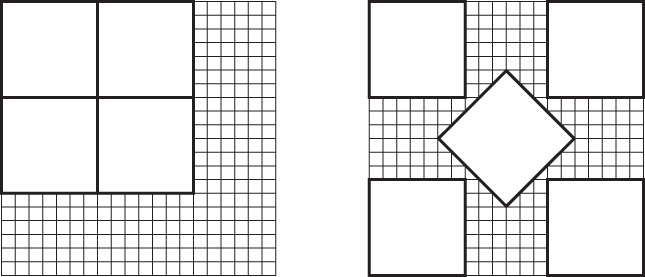
Figure 12.4: If you don't allow rotation, some solutions are impossible.
A common variation of the cutting stock problem involves a single very long piece of stock, such as a roll of paper. The goal is to minimize the number of linear inches of stock used.
Knapsack
In the knapsack problem, you are given a set of objects that have weights and values and a knapsack that holds a certain amount of weight. Your goal is to find the items with the maximum value that will fit in the knapsack. For example, you might fill the knapsack with a few heavy items that have high values, or you may be better off filling it with lots of lighter items that have lower values.
The knapsack problem is similar to the partition problem, in which you try to divide the items into two groups—one with items to go into the knapsack and one with items to remain outside. In the knapsack problem, the goal is to make the first group as valuable as possible and also to ensure that the first group fits inside the knapsack.
Because the knapsack's basic structure is similar to that of the partition problem, you can use a similar decision tree. The main differences are that not all assignments are legal due to the weight constraint, and the goal is different.
The same techniques that work well with the partition problem also work with the knapsack problem. Random solutions, improved solutions, and simulated annealing work in much the same way as they do for the partition problem.
Branch and bound could stop examining a partial solution if its total weight already exceeded the knapsack's capacity.
Branch and bound could also stop if the total value of the unconsidered items was insufficient to raise the current solution's value enough to beat the best solution found so far. For example, suppose that you've found a solution worth $100 and you're examining a partial solution that has a value of $50. If the total value of all the remaining items is only $20, then you cannot improve this solution enough to beat the current best solution.
At each step, a hill-climbing heuristic would add to the solution the highest-value item that could still fit in the knapsack.
A sorted hill-climbing heuristic might consider the items in order of decreasing weight so that later selections could fill in any remaining room in the knapsack.
Probably a better sorted hill-climbing heuristic would consider the items in order of decreasing value-to-weight ratio, so it would first consider the items worth the most dollars per pound (or whatever the units are).
The decision tree for a knapsack problem with N items contains 2N leaf nodes, so this isn't an easy problem, but at least you can try some heuristics.
Traveling Salesman Problem
Suppose that you're a traveling salesperson who must visit certain locations on a map and then return to your starting point. In the traveling salesman problem (TSP), you must visit those locations in an order that minimizes the total distance covered.
To model this problem as a decision tree, the Kth level of the tree corresponds to selecting an item to visit the Kth location in the completed tour. If there are N locations to visit, the root node has N branches, corresponding to visiting each of the locations first. The nodes at the second level of the tree have N – 1 branches, corresponding to visiting any of the locations not yet visited. The nodes at the third level of the tree have N – 2 branches and so on to the leaves, which have no branches. The total number of leaves in the tree would be ![]() .
.
This tree is so big that you need to use heuristics to find good solutions for all but the tiniest problems.
Satisfiability
Given a logical statement such as “A and B or (A and not C),” the satisfiability problem (SAT) is to decide whether there is a way to assign the values true and false to the variables A, B, and C to make the statement true. A related problem asks you to find such an assignment.
You can model this problem with a binary decision tree in which the left and right branches represent setting a variable to true or false. Each leaf node represents an assignment of values to all of the variables and determines whether the statement as a whole is true or false.
This problem is harder than the partition problem because there are no approximate solutions. Any leaf node makes the statement either true or false. The statement cannot be “approximately true.” (However, if you use probabilistic logic, in which variables have probabilities of truth rather than being definitely true or false, you might be able to find a way to make the statement probably true.)
A random search of the tree may find a solution, but if you don't find a solution, you cannot conclude that there isn't one.
You can try to improve random solutions. Unfortunately, any change makes the statement either true or not, so there's no way that you can improve the solution gradually. This means you cannot really use the path improvement strategy described earlier. Because you can't improve the solution gradually, you also can't use simulated annealing or hill climbing. In general, you also cannot tell if a partial assignment makes the statement false, so you can't use branch and bound either.
With exhaustive and random search as your only real options, you can solve satisfiability for only relatively small problems.
SAT is related to the 3-satisfiability problem (3SAT). In 3SAT, the logical statement consists of terms combined with the And operator. Each term involves three variables, or their negations combined with Or. For example, the statement “(A or B or not C) and (B or not A or D)” is in the 3SAT format.
With some work that is far outside the scope of this book, you can show that SAT and 3SAT are equivalent, so they are equally difficult to solve.
Note that the same kind of decision tree will solve either version of the problem.
Swarm Intelligence
Swarm intelligence (SI) is the result of a distributed collection of mostly independent objects or processes. Typically, an SI system consists of a group of very simple objects that interact with their environment and other nearby objects. Most SI systems are motivated by analogies to patterns found in nature, such as ant exploration, bee foraging, bird flocking, and fish schooling.
Swarm intelligence provides an alternative to decision tree searching. Most swarm algorithms provide what seems to be a chaotic search of a solution space, although many of the algorithms use the same basic techniques used by more organized-seeming algorithms. For example, some SI algorithms use hill climbing or incremental improvement strategies.
You can also adapt some SI strategies to work directly on decision trees. For example, you could make a group of ants crawl randomly across a decision tree.
Note that there are often other ways to solve a particular problem. For example, you can use a particle swarm to find the approximate minimum point on a graph, but you may also be able to use calculus to find the minimum exactly.
Swarm intelligence is still useful, however, for several reasons. First, you can apply SI to problems even when an analytical approach is difficult. SI may also apply when you're working with data generated by some real-world process, so a closed-form solution is impossible. SI is also often applicable to a wide range of problems with only slight modification. Finally, swarm intelligence is just plain interesting.
The following sections describe some of the most common approaches for building SI systems.
Ant Colony Optimization
In nature, ants forage by moving in a more or less straight line away from the nest. At some distance, the ant begins making a series of random turns to search for food. When an ant finds a good food source, it returns to the nest.
As it walks, the ant leaves behind a trail of pheromones to aid in navigation. When a randomly wandering ant crosses a pheromone trail, there is some probability that it will turn and follow that trail, adding its own pheromones. If the food source is desirable enough, many ants will eventually follow the trail and build a pheromone superhighway that strongly encourages other ants to follow it. Even if an ant is following a strong pheromone trail, however, there is a chance that it will leave the trail and explore new territory.
General Optimization
One simple ant colony optimization strategy might launch software “ants” (objects) into different parts of a search space. They would then return to the nest (main program) with an estimate of the quality of the solutions they found. The nest would then send more ants to the most profitable-looking areas for further investigation.
Traveling Salesman
The ant colony approach has been used to find solutions to the traveling salesman problem. The algorithm launches ants into the network, and those ants obey the following simple rules:
- Each ant must visit every node exactly once.
- Ants pick the next node to visit randomly using the following rules:
- Ants pick nearby nodes with a greater probability than farther nodes.
- Ants pick links that are marked with more “pheromone” with greater probability
- When an ant crosses a link, it marks that link with pheromone.
- After an ant finishes its tour, it places more pheromone along its path if that path was relatively short.
The idea behind the pheromones in this approach is that, if a link is used by many paths, then it is probably an important link, so it should also be used by other paths. The more a path is used, the more pheromone it picks up so the more it is used in the future.
Bees Algorithm
The bees algorithm is fairly similar to an ant colony algorithm but without the pheromones. In a beehive, scouts roam randomly around the hive. When a scout finds a promising food source, it returns to the hive, goes to a special area called the dance floor, and does a “waggle dance” to tell forager bees where the food is. The bee adjusts the duration of the dance to indicate the quality of the food. Better food sources lead to longer dances and longer dances recruit more foragers.
In a program, scouts (objects) visit different areas in the solution space and assess the quality of the solutions they find. Next, foragers (other objects) are recruited based on the quality of the solutions and they explore the most promising areas more thoroughly.
A group of foragers examines its assigned area looking for an improved solution. The search area shrinks around the best solution found over time. Eventually, when the bees can find no improvement in an area, the best solution is recorded, and that area is abandoned.
During the whole process, other scouts continue exploring other parts of the solution space to see if they can find other promising areas to search.
Swarm Simulation
In a swarm simulation, the program uses simple rules to make particles behave as if they are in a swarm or flock. For example, the swarm might mimic the behavior of a flock of birds flying between buildings, a crowd of people running through streets, or a school of fish chasing a food source.
One of the main reasons why swarm simulations were invented was simply to study swarms, although they can be used in optimization problems as a sort of parallel hill climbing technique.
Boids
In 1986, Craig Reynolds built an artificial life program named Boids (short for “bird-oid object”) to simulate bird flocking. The original Boids program used three basic steering behaviors to control the boid objects.
- Separation rule: The boids steer away from their neighbors to avoid overcrowding.
- Alignment rule: The boids steer so that they point more closely to the average direction of their neighbors.
- Cohesion rule: The boids steer closer to the average position of their neighbors to keep the flock together.
A particular boid only considers flockmates that lie within a certain distance of the boid and that are within a set angular distance of the direction that the boid is facing. (It cannot see boids that are behind it.)
Figure 12.5 shows a boid evaluating its neighbors. The white boid's neighbors are those within the shaded area. Those boids are within the neighborhood distance indicated by the dashed circle and within a specified angle (in this case a 135° span) of the boid's direction.

Figure 12.5: A boid can see neighbors only within a certain distance and within a certain angle of the boid's direction.
The separation rule adds vectors, pushing the boid away from its neighbors. In Figure 12.5, those vectors are indicated by the thin arrows pointing away from neighbors toward the boid in the center.
The alignment rule makes the boid point more in the same direction as the neighbors. In Figure 12.5, the center boid should turn slightly to the left as indicated by the curved arrow.
The cohesion rule makes the boid more toward the average position of the neighbors. In Figure 12.5, the average position is indicated by a small black dot. The heavy arrow pointing away from the center boid shows this vector's direction.
To simulate movement, each boid has a position (x, y) and a velocity vector <vx, vy>. After each time step, the boid updates its position by adding the velocity vector to the position to get its new position ![]() .
.
In practice, the velocity might be stored in pixels per second. In that case, the program would multiply the vector's components by the elapsed time since the boid was last moved. For example, if 0.1 seconds have elapsed, then the boid's new position would be ![]() . That allows the program to update the boids' positions frequently to provide a smooth animation.
. That allows the program to update the boids' positions frequently to provide a smooth animation.
To produce a frame in the animation, the program calculates the vectors defined by the separation, alignment, and cohesion rules. It scales those vectors by the elapsed time and then multiplies them by weights. For example, a particular simulation might use a relatively small weight for separation and a larger weight for cohesion to produce a more closely spaced flock. The program would then add the weighted vectors to the boid's velocity and then use the velocity to update its position.
There are many ways that you could modify the original rules used by Craig Reynolds. For example, you could allow a boid to see neighbors behind it. The result is still reasonably good, and the code is simpler.
Pseudoclassical Mechanics
Another approach to flock simulation that has given me good results mimics classical mechanics. Each boid has a mass, and those masses contribute forces in various directions—almost as if the boids were planets interacting with each other gravitationally.
The program uses the forces to update a boid's velocity by using the equation ![]() . Here
. Here ![]() is a force vector that you are applying to the boid,
is a force vector that you are applying to the boid, ![]() is the boid's mass, and
is the boid's mass, and ![]() is the resulting acceleration. You add up the accelerations because of all the boid's neighbors, adjust for the elapsed time, and then use the result to update the boid's velocity. You then use the velocity to update the boid's position as before.
is the resulting acceleration. You add up the accelerations because of all the boid's neighbors, adjust for the elapsed time, and then use the result to update the boid's velocity. You then use the velocity to update the boid's position as before.
The cohesion forces point from the boid you are updating toward each of the other boids. The force exerted by another boid is determined by the equation ![]() . Here
. Here ![]() is the resulting force,
is the resulting force, ![]() and
and ![]() are the masses of the two boids, and
are the masses of the two boids, and ![]() is the distance between them.
is the distance between them.
This equation means that the force exerted by a boid drops off quickly as the distance between boids increases, so boids close at hand exert more force than those that are farther away. This means that in this model you consider all of the other boids, not only those within a certain distance. The boids that are far away contribute little to the net force, so they are effectively ignored anyway.
The separation forces point from another boid toward the boid that you are updating, so it pushes the boids apart. This force is determined by the equation ![]() . Because the result is divided by the cube of the distance between the boids, the force drops off quickly. At small distances, the force can be strong (if you give it a large weight). At larger distances, this force shrinks, and the cohesion force dominates so that it can hold the flock together.
. Because the result is divided by the cube of the distance between the boids, the force drops off quickly. At small distances, the force can be strong (if you give it a large weight). At larger distances, this force shrinks, and the cohesion force dominates so that it can hold the flock together.
This model doesn't use the alignment rule, although you could add it if you like.
Goals and Obstacles
Whichever flocking model you use, it's relatively easy to add goals for the flock to chase and obstacles for it to avoid.
To add a goal, create an object that acts much like a boid but that contributes a strong cohesion component and little or no alignment and separation components. That will make the flock steer toward the object.
Conversely, to create an obstacle, make an object that contributes a strong separation component (at least when a boid is close) and little or no alignment and cohesion components. That will make boids avoid the obstacle.
Summary
Decision trees are a powerful tool for approaching complex problems, but they are not the best approach for every problem. For example, you could model the eight queens problem described in Chapter 15 with a decision tree that was eight levels tall and that had 64 branches per node, giving a total of ![]() leaf nodes. By taking advantage of the problem's structure, however, you can eliminate most of the tree's branches without exploring them and examine only 113 board positions. Thinking about the problem as a general decision tree may be a mistake, because it might make you miss the simplifications that let you solve the problem efficiently.
leaf nodes. By taking advantage of the problem's structure, however, you can eliminate most of the tree's branches without exploring them and examine only 113 board positions. Thinking about the problem as a general decision tree may be a mistake, because it might make you miss the simplifications that let you solve the problem efficiently.
Still, decision trees are a powerful technique that you should at least consider if you don't know of a better approach to a problem. Swarm algorithms may sometimes provide another approach to finding solutions in large solution spaces such as decision trees. They can be particularly effective when the problem doesn't have much structure that can help you narrow the search.
This chapter and the previous two described trees and algorithms that build, maintain, and search trees. The next two chapters discuss networks. Like trees, networks are linked data structures. Unlike trees, networks are not hierarchical, so they can contain loops. That makes them a bit more complicated than trees, but it also lets them model and solve some interesting problems that trees can't.
Exercises
You can find the answers to these exercises in Appendix B. Asterisks indicate particularly difficult problems.
- Write a program that exhaustively searches the tic-tac-toe game tree and counts the number of times X wins, O wins, and the game ends in a tie. What are those counts, and what is the total number of games possible? Do the numbers give an advantage to one player or the other?
- Modify the programs you wrote for Exercise 1 so that the user can place one or more initial pieces on a tic-tac-toe board and then count the number of possible X wins, O wins, and ties from that point. How many total games are possible starting from each of the nine initial moves by X? (Do you need to calculate all nine?)
- Write a program that lets the player play tic-tac-toe against the computer. Let the player be either X or O. Provide three skill levels: Random (the computer moves randomly), Beginner (the computer uses minimax with only three levels of recursion), and Expert (the computer uses a full minimax search).
- Write a program that uses exhaustive search to solve the optimizing partition problem. Allow the user to click a button to create a list of random weights between bounds set by the user. Also allow the user to check a box indicating whether the algorithm is allowed to short circuit and stop early.
- Extend the program that you wrote for the preceding problem so that you can perform branch and bound with and without short circuits.
- *Use the program you wrote for Exercise 4 to solve the partition problem using exhaustive search and branch and bound with the values 1 through 5, 1 through 6, 1 through 7, and so on, up to 1 through 25. Then graph the number of nodes visited versus the number of weights being partitioned for the two methods. Finally, on a separate graph, show the logarithm of the number of nodes visited versus the number of weights for the results. What can you conclude about the number of nodes visited for the two methods?
- Extend the program that you wrote for Exercise 5 to use a random heuristic to find solutions.
- Extend the program that you wrote for the preceding problem to use an improvement heuristic to find solutions.
- What groups would a partitioning program find if it used the hill-climbing heuristic for the weights {7, 9, 7, 6, 7, 7, 5, 7, 5, 6}? What are the groups' total weights and the difference between the total weights? What if the weights are initially sorted in increasing order? In decreasing order? Can you conclude anything about the solution given by the different orderings?
- Repeat the preceding problem for the weights {5, 2, 12, 1, 2, 1}.
- Can you think of a group of weights which when sorted in decreasing order does not lead to the best solution?
- Extend the program that you wrote for Exercise 8 to use a hill-climbing heuristic to find solutions.
- Extend the program that you wrote for the preceding problem to use a sorted hill-climbing heuristic to find solutions.
- *Build a program that uses Craig Reynolds' original Boids rules to simulate a flock. Make the mouse position a goal so that the flock tends to chase the mouse as it moves over the drawing area. What do the boids do if the target mouse position remains stationary?
- *Modify the program that you built for the preceding exercise to add people as obstacles. When the user clicks the drawing area, place a person at that point and make the boids avoid it.
- *Build a program that uses pseudoclassical mechanics to simulate a flock. Make the mouse position a goal so that the flock tends to chase the mouse as it moves over the drawing area. What do the boids do if the target mouse position remains stationary?
- *Modify the program that you built for the preceding problem to add people as obstacles. When the user clicks the drawing area, place a person at that point and make the boids avoid it.
- *Write a program that uses a swarm to minimize the following function:

Here, r and θ are the polar coordinate values for the point (x, y) in the area −3 ≤ {x, y} ≤ 3. You can use the following functions to calculate r and θ:
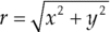

Figure 12.6 shows an image of this function taken from my book WPF 3d: Three-Dimensional Graphics with WPF and C# (Rod Stephens, 2018).

Figure 12.6: Use a swarm of bugs to minimize this strange function.
You can use the following code snippet to calculate this function:
// Return the function's value F(x, y).private double Strange(Point2d point){double r2 = (point.X * point.X + point.Y * point.Y) / 4;double r = Math.Sqrt(r2);double theta = Math.Atan2(point.Y, point.X);double z = 3 * Math.Exp(-r2) *Math.Sin(2 * Math.PI * r) *Math.Cos(3 * theta);return z;}To use the swarm, make a
Bugclass. Give itLocationandVelocityproperties to track its current position, direction, and speed. Also give itBestValueandBestPointproperties to keep track of the best solution that the bug has found.When a timer ticks, the main program should call each bug's
Movemethod. That method should use two accelerations to update the bug's position: a cognition acceleration and a social acceleration. The cognition acceleration should point from the bug's current position toward the best position that it has found. The social acceleration should point from the bug's current position toward the global best position found by any of the bugs.Multiply each acceleration by a weighting factor (set by the user) and a random scale factor between 0 and 1, and then add them to the bug's current velocity. You may need to set a maximum velocity to keep the bugs from running too far away. Then use the result to update the bug's position.
After moving a bug, update its best value and the global best value if appropriate. After a bug has not improved its best value in a certain number of turns, lock its position and don't move it again.
Finally, after each tick, display the bugs, their best positions, and the global best position in different colors. Display locked bugs in a different color. Figure 12.7 shows the SwarmMinimum example program searching for a minimum.

Figure 12.7: Display the bugs, their best positions, and the global best position.