
CHAPTER 13
Basic Network Algorithms
Chapters 10–12 explained trees. This chapter describes a related data structure: the network. Like a tree, a network contains nodes that are connected by links. Unlike the nodes in a tree, however, the nodes in a network don't necessarily have a hierarchical relationship. In particular, the links in a network may create cycles, so a path that follows the links could loop back to its starting position.
This chapter explains networks and some basic network algorithms, such as detecting cycles, finding shortest paths, and finding a tree that is part of the network that includes every node.
Network Terminology
Network terminology isn't quite as complicated as tree terminology, because it doesn't borrow as many terms from genealogy, but it's still worth taking a few minutes to review the relevant terms.
A network consists of a set of nodes connected by links. (Sometimes, particularly when you're working on mathematical algorithms and theorems, a network is called a graph, nodes are called vertices, and links are called edges.) If node A and node B are directly connected by a link, they are adjacent and are called neighbors.
Unlike the case with a tree, a network has no root node, although there may be particular nodes of interest depending on the network. For example, a transportation network might contain special hub nodes where buses, trains, ferries, or other vehicles start and end their routes.
A link can be undirected (you can traverse it in either direction) or directed (you can traverse it in one direction only). A network is called a directed or undirected network depending on what kinds of links it contains.
A path is an alternating sequence of nodes and links through the network from one node to another. Suppose that there is only one link from any node to any adjacent node (in other words, there aren't two links from node A to node B). In that case, you can specify a path by listing either the nodes it visits or the links it uses.
A cycle or loop is a path that returns to its starting point.
As is the case with trees, the number of links that leave a node is called the node's degree. The degree of the network is the largest degree of any of the nodes in it. In a directed network, a node's in-degree and out-degree are the numbers of links entering and leaving the node.
Nodes and links often have data associated with them. For example, nodes often have names, ID numbers, or physical locations such as a latitude and longitude. Links often have associated costs or weights, such as the time it takes to drive across a link in a street network. They may also have maximum capacities, such as the maximum amount of current that you can send over a wire in a circuit network or the maximum number of cars that can cross a link in a street network per unit of time.
A reachable node is one that you can reach from a given node by following links. Depending on the network, you may be unable to reach every node from every other node.
In a directed network, if node B is reachable from node A, nodes A and B are said to be connected. Note that if node A is connected to node B, and node B is connected to node C, then node A must be connected to node C.
A connected component in an undirected network is a set of nodes and links in which every pair of nodes is connected by a path through the set's links. The network is called connected if all of its nodes are connected to each other.
If a directed network's nodes are all mutually connected, then the network is called strongly connected. If a directed network becomes connected when you replace its directed links with undirected links, then the network is called weakly connected.
A subset of a network is called a strongly connected component if it contains a path between any two of its nodes, and it is maximal, so you cannot add another node to the set without breaking its strong connectivity.
Figure 13.1 shows some of the parts of a small directed network. Arrows represent the links, and the arrowheads indicate the links' directions. Undirected links are represented either without arrows or with arrows at both ends.
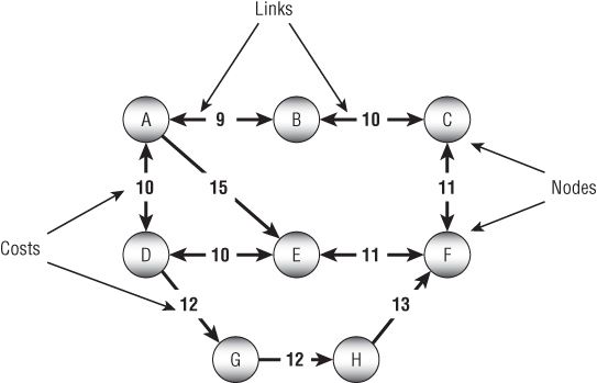
Figure 13.1: In a directed network, arrows show the directions of links.
The numbers on the links are the links' costs. This example assumes that opposite links have the same costs. That need not be the case, but then drawing the network is harder.
The network shown in Figure 13.1 is strongly connected because you can find a path using links from any node to any other node.
Notice that paths between nodes may not be unique. For example, A-E-F and A-B-C-F are both paths from node A to node F.
Table 13.1 summarizes these tree terms to make remembering them a bit easier.
Table 13.1: Summary of Network Terminology
| TERM | MEANING |
| adjacent | If two nodes are connected by a link, then they are adjacent. |
| capacity | The maximum amount of something that can move through a node or link, such as the maximum current that can flow through a wire in an electrical network or the maximum number of cars that can move through a link in a street network per unit of time. |
| connected | In an undirected network, nodes A and B are connected if node B is reachable from node A, and vice versa. An undirected network is connected if every node is reachable from every other node. |
| connected component | A set of nodes that are mutually connected. |
| cost | A link may have an associated cost. Less commonly, a node may have a cost. |
| cycle | A path that returns to its starting point. |
| degree | In an undirected network, the number of links leaving a node. In a directed network, a node has an in-degree and an out-degree. |
| directed | A link is directed if you can traverse it in only one direction. A network is directed if it contains directed links. |
| edge | Link. |
| graph | Network. |
| in-degree | In a directed network, the number of links entering a node. |
| link | An object in a network that represents a relationship between two nodes. Links can be directed or undirected. |
| loop | Cycle. |
| neighbor | Two nodes are neighbors if they are adjacent. |
| node | An object in a network that represents a point-like location. Nodes are connected by links. |
| out-degree | In a directed network, the number of links leaving a node. |
| path | An alternating sequence of nodes and links that leads from one node to another. If there is only one link from any node to an adjacent node, then you can specify a path by listing its nodes or links. |
| reachable node | Node B is reachable from node A if there is a path from node A to node B. |
| strongly connected | A directed network is strongly connected if every node is reachable from every other node. |
| strongly connected component | A maximal subset of a network that contains a path between every pair of its nodes. |
| undirected | A link is undirected if you can traverse it in either direction. A network is undirected if it contains only undirected links. |
| vertex | Node. |
| weakly connected | A directed network is weakly connected if every node is reachable from every other node when you replace the directed links with undirected links. |
| weight | Cost. |
Network Representations
It's fairly easy to use objects to represent a network. You can represent nodes with a Node class.
Exactly how you represent links depends on how you will use them. For example, if you are building a directed network, you can make the links be references to destination nodes that are stored inside the Node class. If the links should have costs or other data, you can also add that to the Node class. The following pseudocode shows a simple Node class for this situation:
Class NodeString: NameList<Node>: NeighborsList<Integer>: CostsEnd Node
This representation works for simple problems, but often it's useful to make a separate class to represent the links. For example, some algorithms, such as the minimal spanning tree algorithm described later in this chapter, build lists of links. If the links are objects, it's easy to place links in a list. If the links are represented by references stored in the node class, it's harder to put them in lists.
The following pseudocode shows Node and Link classes that store links as separate objects for an undirected network:
Class NodeString: NameList<Link>: LinksEnd NodeClass LinkInteger: CostNode: Nodes[2]End Link
Here the Link class contains an array of two Node objects representing the nodes it connects.
In an undirected network, a Link object represents a link between two nodes, and the ordering of the nodes doesn't matter. If a link connects node A and node B, the Link object appears in the Neighbors list for both nodes, so you can follow it in either direction.
Because the order of the nodes in the link's Nodes array doesn't matter, an algorithm trying to find a neighbor must compare the current node to the link's Nodes entries to see which one is the neighbor. For example, if an algorithm is trying to find the neighbors of node A, it must look at a link's Nodes array to see which entry is node A and which entry is the neighbor.
In a directed network, the link class only really needs to know its destination node. The following pseudocode shows classes for this situation:
Class NodeString: NameList<Link>: LinksEnd NodeClass LinkInteger: CostNode: ToNodeEnd Link
However, it may still be handy to make the link class contain references to both of its nodes. For example, if the network's nodes have spatial locations, and the links have references to their source and destination nodes, then it is easier for the links to draw themselves. If the links store only references to their destination nodes, then the node objects must pass extra information to a link to let it draw itself.
If you use a link class that uses the Nodes array, you can store the node's source node in the array's first entry and its destination node in the array's second entry.
The best way to store a network in a file depends on the tools available in your programming environment. For example, even though XML is a hierarchical language and works most naturally with hierarchical data structures such as trees, some XML libraries can also save and load network data.
To keep things simple, the examples that are available for download use a simple text file structure. The file begins with the number of nodes in the network. After that, the file contains one line of text per node.
Each node's line contains the node's name and its x- and y-coordinates. Following that is a series of entries for the node's links. Each link's entry includes the index of the destination node, the link's cost, and the link's capacity.
The following lines show the format:
number_of_nodesname,x,y,to_node,cost,capacity,to_node,cost,capacity,…name,x,y,to_node,cost,capacity,to_node,cost,capacity,…name,x,y,to_node,cost,capacity,to_node,cost,capacity,……
For example, the following is a file representing the network shown in Figure 13.2:
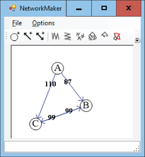
Figure 13.2: This network contains four links—two connecting node A to nodes B and C and two connecting node B to node C.
3A,85,41,1,87,1,2,110,4B,138,110,2,99,4C,44,144,1,99,4
The file begins with the number of nodes, 3. It then contains lines representing each node.
The line for node A begins with its name, A. The next two entries give the node's ![]() and
and ![]() coordinates, so this node is at location (85, 41).
coordinates, so this node is at location (85, 41).
The line then contains a sequence of sets of values describing links. The first set of values 1, 87, 1 means that the first link leads to node B (index 1), has a cost of 87, and has a capacity of 1. The second set of values 2, 110, 4 means that the second link leads to node C (index 2), has a cost of 110, and has a capacity of 4.
The file's other lines define nodes B and C and their links.
Traversals
Many algorithms traverse a network in some way. For example, the spanning tree and shortest path algorithms described later in this chapter all visit the network's nodes.
The following sections describe several algorithms that use different kinds of traversals to solve network problems.
Depth-First Traversal
The preorder traversal algorithm for trees described in Chapter 10 almost works for networks. The following pseudocode shows the almost correct algorithm modified slightly to use a network node class:
Traverse()<Process node>For Each link In Linkslink.Nodes[1].TraverseNext linkEnd Traverse
The method first processes the current node. It then loops through the node's links and recursively calls itself to process each link's destination node.
This would work except for one serious problem. Unlike trees, networks may contain cycles. If a network contains a cycle, this algorithm will end up in an infinite loop, recursively following the cycle.
One solution to this problem is to give the algorithm a way to tell whether it has visited a node before. An easy way to do that is to add a Visited property to the Node class. The following pseudocode shows the algorithm rewritten to use a Visited property:
Traverse()<Process node>Visited = TrueFor Each link In LinksIf (Not link.Nodes[1].Visited) Thenlink.Nodes[1].TraverseEnd IfNext linkEnd Traverse
Now the algorithm visits the current node and sets its Visited property to True. It then loops through the node's links. If the Visited property of the link's destination node is False, the algorithm recursively calls itself to process that destination node.
This version works, but it may lead to very deep levels of recursion. If a network contains N nodes, the algorithm might call itself N times. If N is large, that could exhaust the program's stack space and make the program crash.
You can avoid this problem if you use the techniques described in Chapter 15 to remove the recursion. The following pseudocode shows a version of the algorithm that uses a stack instead of recursion:
DepthFirstTraverse(Node: start_node)// Visit this node.start_node.Visited = True// Make a stack and put the start node in it.Stack(Of Node): stackstack.Push(start_node)// Repeat as long as the stack isn't empty.While <stack isn't empty>// Get the next node from the stack.Node node = stack.Pop()// Process the node's links.For Each link In node.Links// Use the link only if the destination// node hasn't been visited.If (Not link.Nodes[1].Visited) Then// Mark the node as visited.link.Nodes[1].Visited = True// Push the node onto the stack.stack.Push(link.Nodes[1])End IfNext linkLoop // Continue processing the stack until emptyEnd DepthFirstTraverse
This algorithm visits the start node and pushes it onto a stack. Then, as long as the stack isn't empty, it pops the next node off the stack and processes it.
To process a node, the algorithm examines the node's links. If a link's destination node has not been visited, the algorithm marks it as visited and adds it to the stack for later processing.
Because of the way this algorithm pushes nodes onto a stack, it traverses the network in a depth-first order. To see why, suppose that the algorithm starts at node A and node A has neighbors B1, B2, and so on. When the algorithm processes node A, it pushes the neighbors onto the stack. Later, when it processes neighbor B1, it pushes that node's neighbors C1, C2, and so on, onto the stack. Because the stack returns items in last-in, first-out order, the algorithm processes the C nodes before it processes the B nodes. As it continues, the algorithm moves quickly through the network, traveling long distances away from the start node A before it gets back to processing that node's closer neighbors.
Because the traversal visits nodes far from the root node before it visits all the ones that are closer to the root, this is called a depth-first traversal.
Figure 13.3 shows a depth-first traversal with the nodes labeled according to the order in which they were traversed.
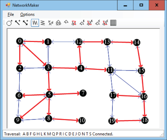
Figure 13.3: In a depth-first traversal, some nodes far from the start node are visited before some nodes that are closer to the start node.
With some work, you can figure out how the nodes were added to the traversal. The algorithm started with the node labeled 0. It then added the nodes labeled 1, 2, and 3 to its stack.
Because node 3 was added to the stack last, it was processed next, and the algorithm added nodes 4 and 5 to the stack. Because node 5 was added last, the algorithm processed it next and added nodes 6, 7, 8, and 9 to the stack.
If you like, you can continue studying Figure 13.3 to figure out why the algorithm visited the nodes in the order it did. At this point, however, you should be able to see how some nodes far from the start node are processed before some of the nodes closer to the start node. For example, node 10, which is four links away from the start node, is visited before nodes 11 and 12, which are only three links away from the start node.
Breadth-First Traversal
In some algorithms, it is better to visit nodes closer to the start node before visiting the nodes that are farther away. The previous algorithm visited some nodes far from the start node before it visited some closer nodes because it used a stack to process the nodes. If you use a queue instead of a stack, then the nodes are processed in first-in, first-out order, and the nodes closer to the start node are processed first.
Because this algorithm visits all of a node's neighbors before it visits any other nodes, this is called a breadth-first traversal. Figure 13.4 shows a breadth-first traversal with the nodes labeled according to the order in which they were traversed.
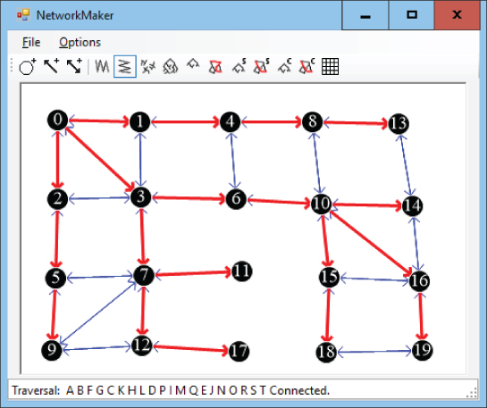
Figure 13.4: In a breadth-first traversal, nodes close to the starting node are visited before those that are farther away.
As with the depth-first traversal, you can study Figure 13.4 to see how the algorithm visited the network's nodes. The algorithm started with the node labeled 0. It then added its neighbors labeled 1, 2, and 3 to its queue.
Because the queue returns items in first-in, first-out order, the algorithm next processes node 1 and adds its neighbors to the queue. The only neighbor of that node that has not been visited yet is node 4.
Next the algorithm removes node 2 from the queue and adds its neighbor, marked 5, to the queue. It then removes the node marked 3 from the queue and adds its neighbors 6 and 7 to the queue.
If you like, you can continue studying Figure 13.4 to determine why the algorithm visited the nodes in the order that it did. At this point, however, you should be able to see that all of the nodes closest to the start node were visited before any of the nodes farther away.
Connectivity Testing
The traversal algorithms described in the previous two sections immediately lead to a couple other algorithms with only minor modifications. For example, a traversal algorithm visits all of the nodes that are reachable from the start node. For an undirected network, this means that it visits every node in the network if the network is connected. This leads to the following simple algorithm to determine whether an undirected network is connected:
Boolean: IsConnected(Node: start_node)// Traverse the network starting from start_node.Traverse(start_node)// See if any node has not been visited.For Each node In <all nodes>If (Not node.Visited) Then Return FalseNext node// All nodes were visited, so the network is connected.Return TrueEnd IsConnected
This algorithm uses the previous traversal algorithm and then checks each node's Visited property to see if it was visited.
You can extend this algorithm to find all of the network's connected components. Simply use the traversal algorithm repeatedly starting at previously unvisited nodes until you visit all of the nodes. The following pseudocode shows an algorithm that uses a depth-first traversal to find the network's connected components:
List(Of List(Of Node)): GetConnectedComponents// Keep track of the number of nodes visited.Integer: num_visited = 0;// Make the result list of lists.List(Of List(Of Node)): components// Repeat until all nodes are in a connected component.While (num_visited < <number of nodes>)// Find a node that hasn't been visited.Node: start_node = <first node not yet visited>// Add the start node to the stack.Stack(Of Node): stackstack.Push(start_node)start_node.Visited = Truenum_visited = num_visited + 1// Add the node to a new connected component.List(Of Node): componentcomponents.Add(component)component.Add(start_node)// Process the stack until it's empty.While <stack isn't empty>// Get the next node from the stack.Node: node = stack.Pop()// Process the node's links.For Each link In node.Links// Use the link only if the destination// node hasn't been visited.If (Not link.Nodes[1].Visited) Then// Mark the node as visited.link.Nodes[1].Visited = True// Mark the link as part of the tree.link.Visited = Truenum_visited = num_visited + 1// Add the node to the current connected component.component.Add(link.Nodes[1])// Push the node onto the stack.stack.Push(link.Nodes[1])End IfNext linkEnd // While <stack isn't empty>Loop // While (num_visited < <number of nodes>)// Return the components.Return componentsEnd GetConnectedComponents
This algorithm returns a list of lists, each holding the nodes in a connected component. It starts by making the variable num_visited to keep track of how many nodes have been visited. It then makes the list of lists that it will return.
The algorithm then enters a loop that continues as long as it has not visited every node. Inside the loop, the program finds a node that has not yet been visited, adds it to a stack as in the traversal algorithm, and also adds it to a new list of nodes that represent the network's connected components.
The algorithm then enters a loop similar to the one used by the earlier traversal algorithm used to process the stack until it is empty. The only real difference is that this algorithm adds the nodes it visits to the list that it is currently building in addition to adding them to the stack.
When the stack is empty, the algorithm has visited all of the nodes that are connected to the latest start node. At that point, it finds another node that hasn't been visited and starts again.
When every node has been visited, the algorithm returns the list of connected components.
Spanning Trees
If an undirected network is connected, then you can make a tree rooted at any node showing a path from the root to every other node in the network. This tree is called a spanning tree because it spans all of the nodes in the network.
For example, Figure 13.5 shows a spanning tree rooted at node H. If you follow the thicker links, you can trace a path from the root node H to any other node in the network. For example, the path to node M visits nodes H, C, B, A, F, K, L, and M.
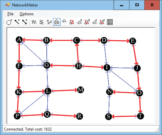
Figure 13.5: A spanning tree connects all of the nodes in a network.
The traversal algorithms described earlier actually find spanning trees, but they don't record the links that are used in the tree. To modify the previous algorithms to record the links used, simply add the following lines right after the statement that marks a new node as visited:
// Mark the link as part of the spanning tree.link.Visited = True
The algorithm starts with the root node in the spanning tree. At each step, it picks another node that is adjacent to the spanning tree and adds it to the tree. The new algorithm simply records which links were used to connect the nodes to the growing spanning tree.
Minimal Spanning Trees
The spanning tree algorithm described in the preceding section could use many different combinations of links to connect all of the network's nodes, so many spanning trees are possible.
A spanning tree that has the least possible cost is called a minimal spanning tree. Note that a network may have more than one minimal spanning tree.
The following steps describe a simple high-level algorithm for finding a minimal spanning tree with root node R:
- Add the root node R to the initial spanning tree.
- Repeat until every node is in the spanning tree:
- Find a least-cost link that connects a node in the spanning tree to a node that is not yet in the spanning tree.
- Add that link's destination node to the spanning tree.
This is an example of a greedy algorithm because at each step it selects a link that has the least possible cost. By making the best choices locally, it achieves the best solution globally.
For example, consider the network shown on the left in Figure 13.6, and suppose that the bold links and nodes are part of a growing spanning tree rooted at node A. In step 2a, you examine the links that connect nodes in the tree with nodes that are not yet in the tree. In this example, those links have costs 15, 10, 12, and 11. Using the greedy algorithm, you add the least-cost link, which has cost 10, to get the tree on the right.
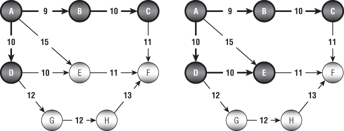
Figure 13.6: At each step, you add to the spanning tree the least-cost link that connects a node in the tree to a node that is not in the tree.
The most time-consuming step in this algorithm is step 2a, which finds the next link to add to the tree. How much time this step takes depends on the approach you use.
One way to find a least-cost link is to loop through the tree's nodes, examining their links to find one that connects to a node outside the tree and that has minimal cost. This is fairly time-consuming because the algorithm must examine the links of the tree's nodes many times, even if they lead to other nodes that are already in the tree.
A better approach is to keep a list of candidate links. When the algorithm adds a node to the growing spanning tree, it also adds any links from that node to a node outside the tree to the candidate list. To find a minimal link, the algorithm looks through the candidate list for the smallest link. As it searches the list, if it finds a link that leads to another node that is already in the tree (because that node was added to the tree after the link was added to the candidate list), the algorithm removes it from the list. That way, the algorithm doesn't need to consider the link again later. When the candidate list is empty, the algorithm is done.
Euclidean Minimum Spanning Trees
The Euclidean minimum spanning tree (EMST) for a set of points is a spanning tree that joins the points with links that have weights equal to their lengths. Another way to think of this is that the EMST connects the points with the smallest total link length. Figure 13.7 shows a program displaying an EMST for a set of points.
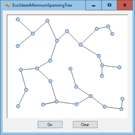
Figure 13.7: An EMST is the cheapest way to connect a set of points.
The EMST is useful for calculating the least expensive way to connect a collection of points. For example, you could use an EMST to build a network of electrical wires, drainage pipes, or telecommunication lines that connect a set of points. In the real world, however, you might prefer to spend a bit more on extra links to provide better throughput or to make the network fault tolerant so that it can continue working even if one of the links breaks.
The most obvious way to build an EMST is to create a network that includes a link between every pair of nodes, set each link's weight equal to its length, and then use the greedy algorithm described in the preceding section to find a minimal spanning tree for the network.
There are faster algorithms for finding an EMST, but they are much more complicated, so I'm not going to describe them here. You can find more information online, for example, at https://wikipedia.org/wiki/Euclidean_minimum_spanning_tree.
Building Mazes
You can use a spanning tree to create a maze relatively easily. First, create an area covered in square rooms separated by walls. Place a node in the middle of each room and connect each node to its north, south, east, and west neighbors. Next, generate a random spanning tree for the nodes. Wherever the tree's links cross through a room's wall, remove that wall.
Figure 13.8 shows a program that used this technique to create a maze. The thin, dark lines show the walls between the maze's rooms. The thick, gray lines show the spanning tree.
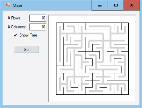
Figure 13.8: You can use a random spanning tree to generate a maze.
You can build the maze's spanning tree almost as you would build any other spanning tree. Pick a random root node and add its links to a candidate list. As long as the candidate list is not empty, pick a random link from the list and add it to the tree as usual.
The only difference between this algorithm and other spanning tree algorithms is that this version picks the next link from the candidate list randomly.
Strongly Connected Components
A subset of nodes in a network is strongly connected if every node in the set is reachable from every other node in the set. A strongly connected component of a network is a maximal strongly connected subset within the network. In other words, it is strongly connected, and if you add any other node to the subset, it is no longer strongly connected.
A network's strongly connected components partition the network. For example, Figure 13.9 shows a network with its strongly connected components circled with dashes.

Figure 13.9: A network's strongly connected components partition the network.
The following section describes one algorithm for finding strongly connected components. The section after that one explains why the algorithm works.
Kosaraju’s Algorithm
In 1978, Johns Hopkins computer science professor Sambasiva Rao Kosaraju proposed a method for finding the strongly connected components of a network. The algorithm is now known as Kosaraju's algorithm. (It's also known as the Kosaraju–Sharir algorithm, partially named after Israeli mathematician and computer scientist Micha Sharir, who independently discovered and published the algorithm in 1981.)
The algorithm is reasonably simple, although understanding why the algorithm works is a bit harder. The following steps outline the algorithm at a high level:
- Preparation: Give the
Nodeclass the following fields:Visited: A Boolean field indicating whether the node has been visited in the first part of the algorithmComponentRoot: ANodethat will represent the strongly connected component to which this node belongsInLinks: A list of links leading into this node
- Initialization: Loop through the nodes and initialize them as follows:
- Set each node's
Visitedfield to false. - Set each node's
ComponentRootfield to null. - Add the node's links to the neighboring nodes'
InLinkslists. - Create an empty
visited_nodeslist to keep track of nodes that have been visited.
- Set each node's
- Visiting: Loop through the nodes and call the recursive
Visitmethod described shortly for each. - Assigning: Loop through the nodes in the
visited_nodeslist and call the recursiveAssignmethod described shortly for each.
The algorithm first performs some setup. The most interesting part of this step is creating an InLinks list for each node. Later the Assign method will use those lists to loop through the nodes' incoming links.
The algorithm then calls the following Visit method for each node:
// Recursively visit nodes that are reachable from this one.Void: Visit(Node: node, List<Node>: visited_nodes)If (node.Visited) Then Returnnode.Visited = TrueFor Each link In node.LinksVisit(link.ToNode, visited_nodes)Next linkvisited_nodes.Insert(0, node)End Visit
The Visit method uses a node's Links list to traverse recursively all of the nodes that are reachable from that node, skipping any nodes that have already been visited.
Note that the method waits until after it has recursively processed a node's outbound links before it adds the node itself to the beginning of the visited_nodes list. That places the node closer to the beginning of the list than any nodes that can be reached from it.
After the visiting step, the algorithm loops through the nodes in the visited_nodes list and calls the following Assign method for each:
// Recursively assign nodes to a component root.Void: Assign(Node: node, Node: root)If (node.ComponentRoot != null) Then Returnnode.ComponentRoot = rootFor Each link In node.InLinksAssign(link.FromNode, root)Next linkEnd Assign
When the method is first called, the node that is passed into it becomes the root node for its connected component. It passes that same root into any recursive calls that the method makes.
For both the initial and recursive calls, the code sets the current node's ComponentRoot field to the component's root node. It then recursively traverses the node's incoming links to assign other nodes to the same component.
When the Assign method has visited every node, then the algorithm is finished, and each node's ComponentRoot field indicates the strongly connected component that contains it.
After executing the algorithm, a program can perform other tasks such as assigning names, numbers, or colors to the nodes in each strongly selected component.
Algorithm Discussion
The key fact that you need to understand to know why Kosaraju's algorithm works is that the nodes in a strongly connected component are exactly those that are reachable both along paths that use forward links and paths that use transpose links. Another way you can state this is by using the following two facts:
- Fact 1 If A and B are in the same strongly connected component, then there is a path PAB from node A to node B using forward links, and there is also a reversed path RAB from node A to node B using reversed links. (There are similar paths and reversed paths between every pair of nodes in the strongly connected component.)
- Fact 2 At least one of the paths PAE or RAE is missing for any node E that lies outside of the strongly connected component that contains node A. In other words, either there is no path PAE or there is no reversed path RAE or there is neither path. (Similarly, there is no path PEA or there is no reversed path REA or there is neither of those paths.)
To see why Fact 1 is true, suppose that nodes A and B are in the same strongly connected component. Then there must be a path PAB from node A to node B and another path PBA from node B to node A. (That's just the definition of a strongly connected component.) Now let's reverse the paths. The reverse of path PAB gives a reverse path RBA that connects node B to node A along the reversed links. Similarly, the reverse of path PBA gives a reverse path RAB that connects node A to node B along the reversed links. This shows that the paths PAB and RAB exist.
To see why Fact 2 is true, suppose that node E is not in the same strongly connected component as node A. Because the two are not in the same strongly connected component, then there is either no path PAE or there is no path PEA. In that case, either one or both of the reversed paths REA or PAE must also be missing, and that's what Fact 2 says.
If you look again at Figure 13.9, you'll see that node E is not part of the strongly connected component {A, B, C, D} because while there are paths from those nodes to node E, there are no paths between node E and any of those nodes. If you study the figure a bit more, you can also verify that there are paths and reversed paths between any pair of nodes in the strongly connected component {A, B, C, D}.
All of this leads to an algorithm for finding a strongly connected component. Start at node A and traverse the network as far as possible following forward links. Then start at node A again, this time traversing the network using reversed links. The strongly connected component that contains node A consists of the nodes that you reach in both traversals. The only remaining task is to figure out how to perform those traversals efficiently. That's where Kosaraju's algorithm comes in.
The algorithm first performs a traversal using forward links. It inserts each node at the beginning of the visited_nodes list, so it comes before the nodes that were visited starting at that node.
Next, the algorithm visits the nodes in the list and traverses the network using reversed links. Eventually, the Assign method reaches a dead end, either because it hits nodes that have already been assigned or because it runs out of transpose links to follow. In either case, it has finished building that strongly connected component.
To get a better idea about how that works, it's worth looking more closely at an example. Consider again the network shown in Figure 13.9 and repeated here in Figure 13.10.
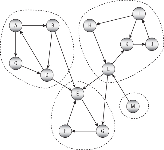
Figure 13.10: Kosaraju's algorithm traverses the network's links forward and then backward.
When the algorithm visits node A, it follows forward links as far as possible. When it finishes that traversal, the visited_nodes list contains the following nodes. I've highlighted node A to indicate that it started the traversal:
A C B D E G F Notice that these nodes include all the nodes in node A's strongly connected component plus a few extras.
The next nontrivial traversal that the algorithm performs starts at the next unvisited node, which is node H. After that traversal, the visited_nodes list contains the following nodes:
H L K J I A C B D E G F The only remaining nontrivial traversal starts at node M and simply adds that node to the beginning of the list.
M H L K J I A C B D E G F Now the algorithm uses the Assign method to assign nodes. It starts at the first node in the nodes_visited list, which is node M, and it performs a traversal using reversed links. That node has no reversed links, so the traversal goes nowhere, and node M is the only node in its strongly connected component.
The algorithm then calls Assign for the next node in the list, which is node H. The new traversal follows reversed links to assign nodes I, J, K, and L. (Look again at the figure to see which reversed links it follows.) It would visit node M, but that node has already been assigned.
The algorithm continues moving through the nodes_visited list calling Assign for the nodes. The nodes L, K, J, and I have already been assigned, so those calls don't do anything interesting. The next nontrivial call is for node A. That reversed traversal assigns nodes D, B, and C.
The algorithm again passes over some previously assigned nodes and then performs a reversed traversal starting at node E. That traversal assigns nodes F and G. That traversal would also visit nodes B, D, and L (and other nodes accessible from them), but those nodes have already been assigned.
The algorithm finishes looping through the visited_nodes list, finds no more unassigned nodes, and is done.
If you still have trouble visualizing how the algorithm works, you may want to implement it and step through it in a debugger.
Finding Paths
Finding paths in a network is a common task. An everyday example is finding a route from one location to another in a street network.
The following sections describe some algorithms for finding paths through networks.
Finding Any Path
The spanning tree algorithms described earlier in this chapter gave you a method for finding a path between any two nodes in a network. The following steps describe a simple high-level algorithm for finding a path from node A to node B:
- Find a spanning tree rooted at node A.
- Follow the reversed links in the spanning tree from node B to node A.
- Reverse the order in which the links were followed.
The algorithm builds the spanning tree rooted at node A. Then it starts at node B. For each node in its path, it finds the link in the spanning tree that leads to that node. It records that link and moves to the next node in the path.
Unfortunately, finding the link that leads to a particular node in the spanning tree is difficult. Using the spanning tree algorithms described so far, you would need to loop through every link to determine whether it was part of the spanning tree and whether it ended at the current node.
You can solve this problem by making a small change to the spanning tree algorithm. First, add a new FromNode property to the Node class. Then when the spanning tree algorithm marks a node as being in the tree, set that node's FromNode property to the node whose link was used to connect the new node to the tree.
Now to find the path from node B to node A in step 2, you can simply follow the nodes' FromNode properties.
Label-Setting Shortest Paths
The algorithm described in the preceding section finds a path from a start node to a destination node, but it's not necessarily a good path. The path is taken from a spanning tree, and there's no guarantee that it is efficient. Figure 13.11 shows a path from node M to node S. If the link costs are their lengths, then it's not hard to find a shorter path such as ![]() .
.
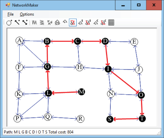
Figure 13.11: A path that follows a spanning tree from one node to another may be inefficient.
A more useful algorithm would find the shortest path between two nodes. Shortest path algorithms are divided into two general categories: label setting and label correcting. This section describes a label-setting algorithm. The next section describes a label-correcting algorithm.
The label-setting algorithm begins at a starting node and creates a spanning tree in a manner that is somewhat similar to how the minimal spanning tree described earlier does this. At each step, the minimal spanning tree algorithm selects the least-cost link that connects a new node to the spanning tree. In contrast, the shortest path algorithm selects a link that adds to the tree a node that is the least distance from the starting node.
To determine which node is the least distance from the starting node, the algorithm labels each node with its distance from the starting node. When it considers a link, it adds the distance to the link's source node to that link's cost, and that determines the current distance to the link's destination node.
When the algorithm has added every node to the spanning tree, it is finished. The paths through the tree show the shortest paths from the starting node to every other node in the network, so this tree is called a shortest path tree.
The following steps describe the algorithm at a high level:
- Set the starting node's distance to 0, and mark it as part of the tree.
- Add the starting node's links to a candidate list of links that could be used to extend the tree.
- While the candidate list is not empty, loop through the list examining the links.
- If a link leads to a node that is already in the tree, remove the link from the candidate list.
- Suppose link L leads from node N1 in the tree to node N2 not yet in the tree. If D1 is the distance to node N1 in the tree and CL is the cost of the link, then you could reach node N2 with distance
 by first going to node N1 and then following the link. Let
 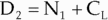 be the possible distance for node N1 that uses this link. As you loop over the links in the candidate list, keep track of the link and node that give the smallest possible distance. Let
  and
and  be the link and node that give the smallest distance
- Set the distance for
 to
to  and mark Nbest as part of the shortest path tree.
 - For all links L leaving node
 if L leads to a node that is not yet in the tree, add L to the candidate list.
For example, consider the network shown on the left in Figure 13.12. Suppose that the bold links and nodes are part of a growing shortest path tree. The tree's nodes are labeled with their distance from the root node, which is labeled 0. The other nodes are labeled with their names.
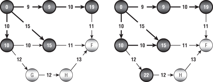
Figure 13.12: At each step, you add to the shortest path tree the link that gives the smallest total distance from the root to a node that is not in the tree.
To add the next link to the tree, examine the links that lead from the tree to a node that is not in the tree and calculate the distance to those nodes. This example has three possible links.
The first leads from the node labeled 19 to node F. The distance from the root node to the node labeled 19 is 19 (that's why it's labeled 19), and this link has cost 11, so the total distance to node F via this link is ![]() .
.
The second link leads from the node labeled 15 to node F. The distance from the root node to the node labeled 15 is 15, and this link has cost 11, so the total distance to node F via this link is ![]() . Notice that this link leads to the same node as the previous one, node F, but this link gives a shorter path to that node.
. Notice that this link leads to the same node as the previous one, node F, but this link gives a shorter path to that node.
The third link leads from the node labeled 10 to node G. The link has cost 12, so the total distance via this link is ![]() . This is the least of the three distances calculated, so this is the link that should be added to the tree. The result is shown on the right in Figure 13.12.
. This is the least of the three distances calculated, so this is the link that should be added to the tree. The result is shown on the right in Figure 13.12.
Figure 13.13 shows a complete shortest path tree built by this algorithm. In this network, the links' costs are their lengths in pixels. Each node is labeled with the order in which it was added to the tree, not its distance from the root. The root node was added first, so it has label 0, the node to its left was added next, so it has label 1, and so on.
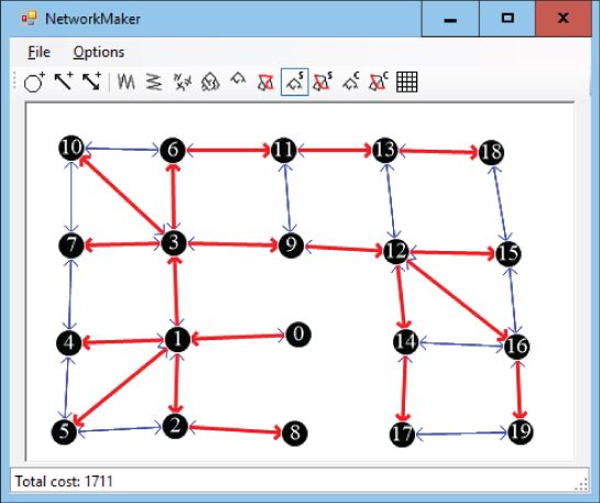
Figure 13.13: A shortest path tree gives the shortest paths from the root node to any node in the network.
Notice how the nodes' labels increase as the distance from the root node increases. This is similar to the ordering in which nodes were added to the tree in a breadth-first traversal. The difference is that the breadth-first traversal added nodes in order of the number of links between the root and the nodes, but this algorithm adds nodes in order of the distance along the links between the root and the nodes.
Having built a shortest path tree, you can follow the nodes' FromNode values to find a backward path from a destination node to the start node, as described in the preceding section.
Figure 13.14 shows the shortest path from node M to node S in the original network. This looks more reasonable than the path shown in Figure 13.11, which used a spanning tree.
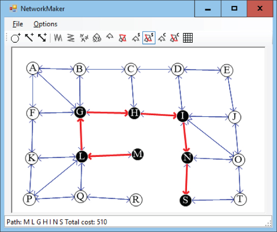
Figure 13.14: A path through a shortest path tree gives the shortest path from the root node to a specific node in the network.
Label-Correcting Shortest Paths
The most time-consuming step in the label-setting shortest path algorithm is finding the next link to add to the shortest path tree. To add a new link to the tree, the algorithm must search through the candidate links to find the one that reaches a new node with the least cost.
An alternative strategy is just to add any of the candidate links to the shortest path tree and label its destination node with its distance to the root as usual.
Later, when the algorithm considers links in the candidate list, it may find a better path to a node that is already in the shortest path tree. In that case, the algorithm updates the node's distance, adds its links back into the candidate list (if they are not already in the list), and continues. Eventually, the algorithm will find no more improved paths and it is done.
In the label-setting algorithm, a node's distance is set only once and never changes. In the label-correcting algorithm, a node's distance is set once but later may be corrected many times.
The following steps describe the algorithm at a high level:
- Set the starting node's distance to 0, and mark it as part of the tree.
- Add the starting node's links to a candidate list of links.
- While the candidate list is not empty:
- Consider the first link in the candidate list.
- Calculate the distance to the link's destination node:
<distance> = <source node distance> + <link cost>. - If the new distance is smaller than the destination node's current distance:
- Update the destination node's distance.
- Add all of the destination node's links to the candidate list.
This algorithm may seem more complicated, but the code is actually shorter, because you don't need to search the candidate list for the best link.
Because this algorithm may change the link leading to a node several times, you cannot simply mark a link as used by the tree and leave it at that. If you did and you needed to change the link that leads into a node, you would need to find its old incoming link and unmark it.
An easier approach is to give the Node class a FromLink property. When you change the link leading to the node, you can update this property.
If you still want to mark the links used by the shortest path tree, first build the tree. Then loop over the nodes, and mark the links stored in their FromLink properties.
Figure 3.15 shows the shortest path tree for a network found by using the label-correcting method. Again, in this network the links' costs are their lengths in pixels. Each node is labeled with the number of times its distance (and FromLink value) was corrected. The root node is labeled 0 because its value was set initially and never changed.
Many of the nodes in Figure 13.15 are labeled 1, meaning that their distances were set once and then never corrected. A few nodes are labeled 2, meaning their values were set and then corrected once.
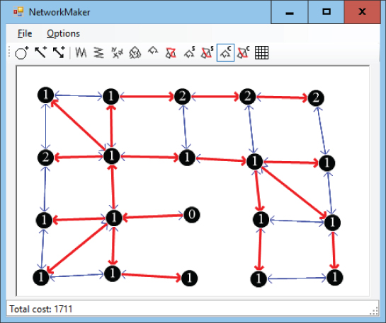
Figure 13.15: In a label-correcting algorithm, some nodes' distances may be corrected several times.
In a large and more complicated network, it is possible that a node's distance might be corrected many times before the shortest path tree is complete.
All-Pairs Shortest Paths
The shortest path algorithms described so far find shortest path trees from a starting node to every other node in the network. Another type of shortest path algorithm asks you to find the shortest path between every pair of nodes in the network.
The Floyd–Warshall algorithm begins with a two-dimensional array named Distance, where Distance[start_node, end_node] is the shortest distance between nodes start_node and end_node.
To build the array, initialize it by setting the diagonal entries, which represent the distance from a node to itself, to 0. Set the entries that represent direct links between two nodes to the cost of the links. Set the array's other values to infinity.
Suppose the Distance array is partially filled, and consider the path within the array from node start_node to node end_node. Suppose also that the path uses only nodes 0, 1, 2, …, via_node – 1 for some value via_node.
The only way adding node via_node could shorten a path is if the improved path visits that node somewhere in the middle. In other words, the path start_node → end_node becomes start_node → via_node followed by via_node → end_node.
To update the Distance array, you examine all pairs of nodes start_node and end_node. If Distance[start_node, end_node] > Distance[start_node, via_node] + Distance[via_node, end_node], then you update the entry by setting Distance[start_node, end_node] equal to the smaller distance.
If you repeat this with ![]() where N is the number of nodes in the network, the
where N is the number of nodes in the network, the Distance array holds the final shortest distance between any two nodes in the network using any of the other nodes as intermediate points on the shortest paths.
So far the algorithm doesn't tell you how to find the shortest path from one node to another. It just explains how to find the shortest distance between the nodes. Fortunately, you can add the path information by making another two-dimensional array named Via.
The Via array keeps track of one of the nodes along the path from one node to another. In other words, Via[start_node, end_node] holds the index of a node that you should visit somewhere along the shortest path from start_node to end_node.
If Via[start_node, end_node] is end_node, then there is a direct link from start_node to end_node, so the shortest path consists of just the node end_node.
If Via[start_node, end_node] is some other node via_node, then you can recursively use the array to find the path from start_node to via_node and then from via_node to end_node. (If this seems a bit confusing, it will probably make more sense when you see the algorithm for using the Via array.)
To build the Via array, initialize all of its entries to –1. Then set Via[start_node, end_node] to end_node if there is a direct link between the nodes.
Now when you build the Distance array and you improve the path start_node → end_node by replacing it with the paths start_node → via_node and via_node → end_node, you need to do one more thing. You must also set Via[start_node, end_node] = via_node to indicate that the shortest path from start_node to end_node goes via the intermediate point via_node.
The following steps describe the full algorithm for building the Distance and Via arrays (assuming that the network contains N nodes):
- Initialize the
Distancearray:- Set
Distance[i, j]= infinity for all entries. - Set
Distance[i, i]= 0 for all to N – 1.
 - If nodes i and j are connected by a link
 , set
, set Distance[i, j]to the cost of that link.
- Set
- Initialize the
Viaarray:- For all i and j:
- If
Distance[i, j]< infinity, setVia[i, j]to j to indicate that the path from i to j goes via node j. - Otherwise, set
Via[i, j]to –1 to indicate that there is no path from node i to node j.
- If
- For all i and j:
- Execute the following nested loops to find improvements:
For via_node = 0 To N - 1For from_node = 0 To N - 1For to_node = 0 To N - 1Integer: new_dist =Distance[from_node, via_node] +Distance[via_node, to_node]If (new_dist < Distance[from_node, to_node]) Then// This is an improved path. Update it.Distance[from_node, to_node] = new_distVia[from_node, to_node] = via_nodeEnd IfNext to_nodeNext from_nodeNext via_node
The via_node loop loops through the indices of nodes that could be intermediate nodes and improve existing paths. After that loop finishes, all of the shortest paths are complete.
The following pseudocode shows how to use the completed Distance and Via arrays to find the nodes in the shortest path from a start node to a destination node:
List(Of Integer): FindPath(Integer: start_node, Integer: end_node)If (Distance[start, end] == infinity) Then// There is no path between these nodes.Return nullEnd If// Get the via node for this path.Integer: via_node = Via[start_node, end_node]// See if there is a direct connection.If (via_node == end_node)// There is a direct connection.// Return a list that contains only end_node.Return { end_node }Else// There is no direct connection.// Return start_node --> via_node plus via_node --> end_node.Return{FindPath(start_node, via_node] +FindPath(via_node, end_node]}End IfEnd FindPath
For example, consider the network shown at the top of Figure 13.16. The upper arrays show how the Distance values change over time, and the bottom arrays show how the Via values change over time. Values that change are highlighted to make them easy to spot.
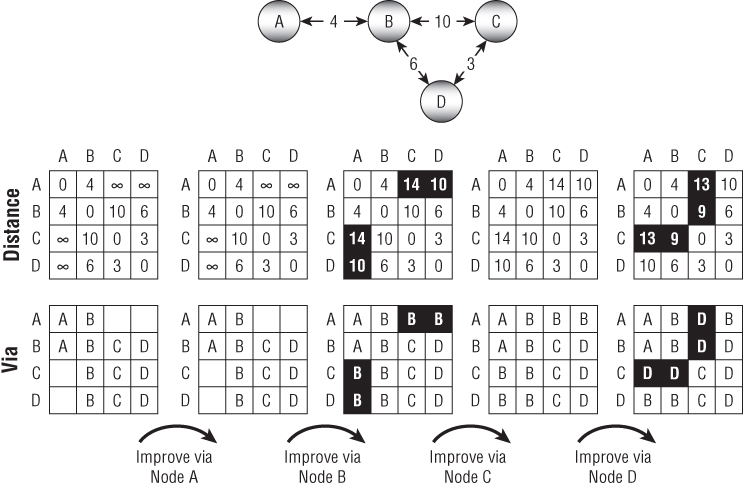
Figure 13.16: The shortest paths between all pairs of nodes in a network can be represented by a Distance array (top arrays) and a Via array (bottom arrays).
The upper-left array shows the initial values in the Distance array. The distance from each node to itself is 0. The distance between two nodes connected by a link is set to the link's cost. For example, the link between node A and node B has cost 4, so Distance[A, B] is 4. (To make the example easier to follow, the names of the nodes are used as if they were array indices.) The remaining entries are set to infinity.
The lower-left array shows the initial values in the Via array. For example, there is a link from node C to node B, so Via[C, B] is B.
After initializing the arrays, the algorithm looks for improvements. First it looks for paths that it can improve by using node A as an intermediate point. Node A is on the end of the network, so it can't improve any paths.
Next the algorithm tries to improve paths by using node B, and it finds four improvements. For example, looking at the second Distance array, you can see that Distance[A, C] is infinity, but Distance[A, B] is 4 and Distance[B, C] is 10, so the path A → C can be improved. To make that improvement, the algorithm sets Distance[A, C] to ![]() and sets
and sets Via[A, C] to the intermediate node B.
If you look at the network, you can follow the changes there. The initial path ![]() had distance set to infinity. The path
had distance set to infinity. The path ![]() is an improvement, and you can see in the network that the total distance for that path is 14.
is an improvement, and you can see in the network that the total distance for that path is 14.
Similarly, you can work through the changes in the paths ![]() and
and ![]() .
.
Next the algorithm tries to improve paths by using node C as an intermediate node. That node doesn't allow any improvements.
Finally, the algorithm tries to improve paths by using node D as an intermediate node. It can use node D to improve the four paths ![]() and
and ![]() .
.
For an example of finding a path through the completed Via array, consider the array on the lower right in Figure 13.16. The following steps describe how to find the path A → C:
Via[A, C]is D, so .
.Via[A, D]is B, so
Via[D, C]is C, so there is a link from node D to node C.Via[A, B]is B, so there is a link from node A to node B.- Finally,
Via[B, D]is D, so there is a link from node B to node D.
The final path travels through nodes B, D, and C, so the full path is ![]()
Figure 13.17 shows the recursive calls.
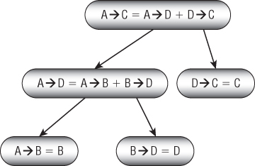
Figure 13.17: To find the path from start_node to end_node with intermediate point via_node, you recursively find the paths from start_node to via_node and from via_node to end_node.
After you create the Distance and Via arrays, you can quickly find the shortest paths between any two points in a network. The downside is that the arrays can take up a lot of room.
For example, a street network for a moderately large city might contain 30,000 nodes, so the arrays would contain ![]() entries. If the entries are 4-byte integers, then the two arrays would occupy a combined 14.4 gigabytes of memory.
entries. If the entries are 4-byte integers, then the two arrays would occupy a combined 14.4 gigabytes of memory.
Even if you can afford to use that much memory, the algorithm for building the arrays uses three nested loops that run from 1 to N, where N is the number of nodes, so the algorithm's total run time is ![]() . If N is 30,000, that's
. If N is 30,000, that's ![]() steps. A computer running 1 million steps per second would need more than 10 months to build the arrays.
steps. A computer running 1 million steps per second would need more than 10 months to build the arrays.
For really big networks, this algorithm is impractical, so you need to use one of the other shortest path algorithms to find paths as needed. If you need to find many paths on a smaller network, perhaps one with only a few hundred nodes, you may be able to use this algorithm to precompute all of the shortest paths and save some time.
Transitivity
Two topics that are closely related to path finding are transitive closure and transitive reduction. In a sense, these ideas are complementary. A networks' transitive closure logically adds links to a network to represent all of its connections directly. In contrast, the transitive reduction removes as many links as possible without changing the network's connectivity.
The following two sections explain transitive closure and transitive reduction in more detail and describe algorithms for performing each.
Transitive Closure
In the transitive closure problem, the goal is to build a data structure that can efficiently determine whether there is a path through a network between any two given nodes. For example, you could construct an array called PathExists where PathExists[A, B] is true if there is a path through the network from node A to node B.
Conceptually, you can think of the closure as adding links to show which nodes are reachable from other nodes. For example, the left side of Figure 13.18 shows a small network. On the right side of the figure, dashed arrows represent new links added to make the network's transitive closure. If there is a path from node X to node Y in the network on the left, then there is a direct link from node X to node Y in the network on the right.
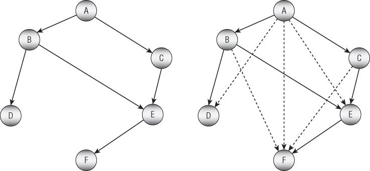
Figure 13.18: In a network's transitive closure, each node is only one link away from every node that it can reach.
There are several methods that you can use to find a transitive closure. The simplest approach is to perform a traversal of the network starting at every node and keep track of all the vertices that the traversal reaches. If the network contains N nodes and E edges, then each traversal takes ![]() steps, so the whole process takes
steps, so the whole process takes ![]() steps. If the network is dense so E is on the order of
steps. If the network is dense so E is on the order of ![]() , then that time is
, then that time is ![]() . That's fast enough for small networks but impractical for large ones.
. That's fast enough for small networks but impractical for large ones.
A second approach is to use the Floyd–Warshall algorithm described in the section “All-Pairs Shortest Paths” earlier in this chapter, which also runs in ![]() time. That algorithm produces an array that gives the shortest distance between every pair of nodes. You can use that array to test reachability between two nodes by checking whether the distance between the nodes is less than infinity.
time. That algorithm produces an array that gives the shortest distance between every pair of nodes. You can use that array to test reachability between two nodes by checking whether the distance between the nodes is less than infinity.
If the network is relatively dense, then a third approach may be useful. Because the network is dense, many of its nodes should be contained in strongly connected components. In that case, you can find those components and then examine the links between them. If there is a link from component A to component B, then all of the nodes in component B are reachable from all of the nodes in component A.
Transitive Reduction
The transitive reduction of a network (which is also known as the minimum equivalent digraph) is another network that has the same nodes but with the fewest possible links that give the same reachablity. In other words, if there is a path between two nodes in the original network, then there is also a path between the same two nodes in the reduced network.
Another way to think of this is to remove as many links as possible from the original network without changing the reachability.
Note that the transitive reduction of an acyclic network is unique. For example, Figure 13.19 shows an acyclic network on the left and its transitive reduction on the right.
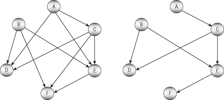
Figure 13.19: An acyclic network's transitive reduction is unique.
If you study the networks shown in Figure 13.19, you'll see that their nodes have the same sets of reachability. Table 13.2 summarizes the networks' reachabilities.
Table 13.2: An Acyclic Network's Reachabilities
| A | B | C | D | E | F | |
| A | X | X | X | X | X | |
| B | X | X | X | X | ||
| C | X | X | X | X | ||
| D | X | |||||
| E | X | |||||
| F | X | X |
In contrast, a cyclic network may have multiple transitive reductions, and even multiple minimum reductions with the fewest possible number of edges. Figure 13.20 shows a cyclic network on the left and two transitive reductions, each containing six links.
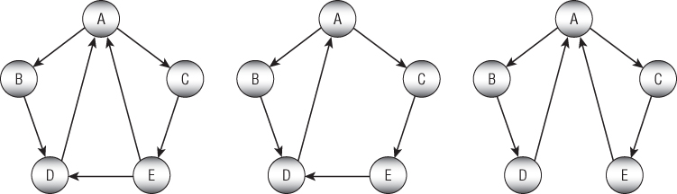
Figure 13.20: A cyclic network's transitive reduction may not be unique.
Note that the transitive reduction of a cyclic network may be unique. For example, both of the transitive closures shown in Figure 13.20 are cyclic networks, and they are their own unique transitive closures.
In general, finding a transitive closure for a network can be difficult, but there are a couple of special cases that are manageable. For example, if the network's links are undirected, then finding a minimal transitive closure is equivalent to finding a minimal spanning tree, and you already know how to do that.
The following two sections explain algorithms that you can use to find a transitive closure for other kinds of networks.
Acyclic Networks
Finding a transitive closure for an acyclic network is relatively simple. The basic idea is to remove links that can be replaced with a composite path consisting of two other paths that visit an intermediate node.
For example, consider the link A → B. If there is a node C such that there are paths A → C and C → B, then the link A → B is unnecessary, and we can remove it from the network without changing the network's reachability. That approach gives the following algorithm for acyclic networks:
// Find the transitive reduction.Void: FindTransitiveReduction(Boolean[,]: reachable)// Remove self-links.For i = 0 To <Number of nodes>reachable[i, i] = False// Remove other unnecessary links.For i = 0 To <Number of nodes> – 1For j = 0 To <Number of nodes> – 1// Consider link i --> j.If (reachable[i, j]) Then// See if there is a node k with paths// i --> k and k --> j.For k = 0 To <Number of nodes> – 1If reachable[i, k] And reachable[k, j] ThenReachable[i, j] = FalseEnd IfEnd IfEnd FindTransitiveReduction
The reachable parameter is a Boolean array where reachable[i, j] is true if there is a path from node i to node j. The code first sets reachable[i, i] to false for all i to remove any self-links between a node and itself.
Next, the algorithm loops over the links between all possible pairs of nodes. For each link i → j, the code loops through all nodes k and checks whether there are paths i → k and k → j. If those paths exist, then the algorithm removes the i → j link.
General Networks
To find a transitive reduction for a general cyclic network, first find the network's strongly connected components. Connect the nodes in each of those components with a directed Hamiltonian cycle. (Basically, make a big loop that connects all of the component's nodes.)
Replace each strongly connected component with a single, condensed node and remove any links that lie within a component. If a link in the original network connected nodes in two different components, add a link connecting the corresponding condensed nodes.
The result is called the original network's condensation. The condensed network is acyclic, so you can use the techniques described in the previous section to find its transitive reduction.
Now use the links that remain in the condensed network's reduction to define the reduced links in the original network.
Shortest Path Modifications
Shortest path algorithms are extremely useful and have many obvious and nonobvious uses including data packet routing, financial transaction planning, network flow calculations, robust infrastructure design, social network analysis, movement planning for artificial intelligence applications, and many more. These days, almost everyone with a smartphone has used these algorithms directly to locate nearby restaurants or to find the fastest route to a friend's house.
Because these algorithms are so important, people have come up with a variety of modifications to their basic designs. The following sections summarize a few possible modifications.
Shape Points
Many networks include two kinds of links: those that represent the network's structure and those that represent its shape. For example, the links in a street network in Manhattan may be short, straight segments, but in parts of San Francisco, the streets curve around considerably. Even if a section of road has no intersections, that doesn't mean it's straight.
For example, Figure 13.21 shows two straight vertical roads and two mostly horizontal curvy roads that follow a river (shown in gray). To draw the curved roads, you would need many points spaced closely together, but the network's topology only depends on the connections among the street sections. In the figure, the large dots show the connections that matter to a shortest path algorithm, and the small dots record the shape of the curvy street sections.
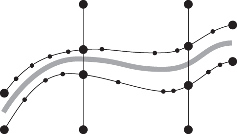
Figure 13.21: Curved streets require many points that don't really matter to the network's connectivity.
To make calculating shortest paths easier, you can build a network that includes only the connections (large dot). For example, each of the curved pieces of road shown in Figure 13.21 would be represented by a single link. An additional ShapePoints list on each link would give the details (small dots) needed to draw the link.
Early Stopping
Label-correcting algorithms are often faster than label-setting algorithms because they don't need to pick the best link to add to the shortest path tree. However, if you know that the destination is relatively close to the starting point, then you may be better off using a label-setting algorithm and then stopping when you reach the destination node.
For example, suppose you want to find a path from your current location in Boston to a restaurant that's about a mile away. A full street network for Boston includes tens of thousands of links, but your path will need to use only a few hundred. In that case, you can use a label-setting algorithm and then stop when you have labeled your destination.
Bidirectional Search
Many shortest path algorithms build a shortest path tree starting at one node and branching out to every other node. Sadly, much of that tree isn't near the shortest path between the start and destination nodes, so a lot of that work is wasted. If the start and destination nodes are close together, then the early stopping strategy described in the preceding section may help. However, if the start and destination nodes are far apart, that method won't help and will probably slow overall performance.
Instead of working outward from a single root node, another approach is to start building shortest path trees from both the start and destination nodes. The searches expand outward from the two nodes in roughly circular patterns until they intersect. At that point, you can find the shortest path through the two trees to connect the two nodes.
Best-First Search
The basic label-correcting, shortest path algorithm adds links to the shortest path tree randomly. Sometimes, you may be able to improve performance if you can quickly pick the best link to add to the tree. For example, you might be able to use the link's direction or the location of the link's end point to get an indication of how well that link will move toward the destination. For example, if the destination node is west of the start node, then you might prefer to use links that point more or less to the west.
In some cases, you might even be able to precalculate link rankings that you can later use to decide which link might be most promising. For example, in a street network, highways tend to be faster than surface streets, so you might give them a higher ranking. Then when the program builds a shortest path tree, it would quickly explore highway links to create paths close to the destination node.
Even then, some prioritized links may be more useful than others. For example, if you're trying to find a path from Los Angeles to Chicago, you probably don't need to explore highway links in Florida.
Turn Penalties and Prohibitions
In many networks, travel is modified by turn penalties. For example, in a street network, left turns generally take longer than right turns, and going straight is usually fastest of all. Left turns are also more dangerous than other maneuvers. UPS even prohibits them (mostly) because they take longer, use extra fuel while the vehicle waits for a chance to turn, and cause more accidents. Giant fleets like those used by UPS, FedEx, and the United States Postal Service drive billions of miles per year, so even a small savings can add up quickly.
Occasionally, a street network will also include turn or direction prohibitions. For example, an intersection may not allow a left turn. Or a turn might be impossible because it would send you down a one-way street in the wrong direction. Sometimes, going straight may even be prohibited if the street is switching from two-way to one-way traffic.
Simple, undirected street networks make it hard for shortest path algorithms to handle turn penalties and prohibitions. For example, if several links meet at an intersection, there's nothing in a simple network to tell the algorithm that it is not allowed to make a particular turn.
The following sections describe some different approaches to handling these situations.
Geometric Calculations
One way to handle turn penalties is to use the network's geometry to add them when you add a new link to the shortest path tree. When the algorithm considers a particular link, it calculates the angle between that link and the one that comes before it in the shortest path tree. For example, it might add a 30-second penalty for right turns greater than 30 degrees and a 60-second penalty for left turns greater than 30 degrees.
This approach has a couple of drawbacks. First, it assumes that all turn penalties can be deduced from the network's geometry. For example, it might assume that a 90-degree left turn deserves a big turn penalty even though the main thoroughfare goes that way, so it should have only a small penalty. This method also cannot handle prohibited turns such as those blocked by a center divider.
A second problem with this method is that this adds a lot of calculations to an otherwise very fast loop, and that will slow performance considerably.
You can work around the second problem (and to an extent the first) by adding a lookup table to each node. When the algorithm wants to use a link out of a node, it uses that table to find the penalty associated with turning from the incoming link to the outgoing link. That table would be large, however, and using it would be relatively slow.
Expanded Node Networks
Another way to model turn penalties is to think of a turn as a separate step while moving through the network. For example, suppose that you want to move from node A to node B, turn left, and arrive at node C. Nodes A, B, and C are already part of the network. What you need to do is to add a new node to represent turning from the A-B link onto the B-C link.
More generally, you can expand a node (in this example, node B) to include subnodes to represent each of the ways that a driver could enter the intersection. You then connect those subnodes with links representing the various turns.
Figure 13.22 shows a simple network on the left. The picture in the middle shows node B expanded to handle turn penalties. The small gray links represent the turns, and their costs give the turn penalties. The extra thick gray link represents the left turn from node A via node B to node C.
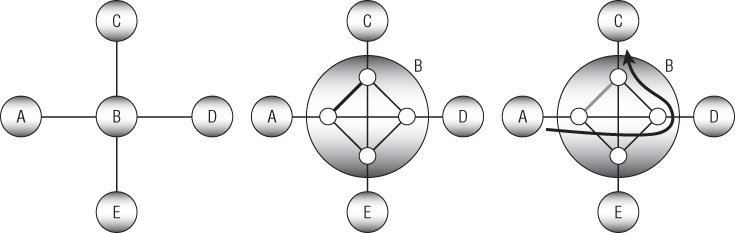
Figure 13.22: You can expand a node to represent turn penalties.
Note that the turn links include two straight links, one vertical and one horizontal, that represent no turn at the intersection. Also note that the links shown here should really be directed links. For example, the thick link represents a left turn from node A to node C, but there should also be a right turn link from node C to node A, and those two links would probably not have the same penalty cost.
This method almost works, but it's not quite restrictive enough to prevent the shortest path algorithm from cheating. The thick path on the right in Figure 13.22 shows how the algorithm can turn left from node A to node C without paying the left turn penalty. The path moves straight through the intersection toward node D, makes a quick about-face, and then follows the link that represents a right turn from node D to node C.
Alternatively, the algorithm could turn right from node A toward node E, make a quick U-turn, and then move straight through the intersection to node C.
To prevent those kinds of shenanigans, you can divide each of the subnodes into two parts: one to represent moving into the original node and one to represent moving out of it. Figure 13.23 shows part of the new structure. Here node B's inbound subnodes are white, and its outbound subnodes are shaded.
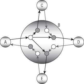
Figure 13.23: Now the algorithm cannot take a shortcut through an intersection and then make a quick about-face.
Figure 13.23 shows only some of the expanded node's links. The paths leading out from node A are dark, and others are gray. There should also be links between every inbound subnode and every outbound subnode that doesn't create a U-turn. For example, there should be links from node D's inbound subnode to the outbound subnodes leading to nodes A and C.
With this new design, if the algorithm tries to move from node A straight through the intersection, then it cannot turn around until it reaches node D.
Interchange Networks
The expanded node technique described in the preceding section allows you to handle turns at a single node. If you want to apply that technique to an entire network, the result will be much larger than the original network.
Another approach is to turn the network inside out so that nodes represent links and links represent turns. This kind of network has many names including interchange network, line network, covering network, edge/vertex dual, edge graph, and several others.
Figure 13.24 shows how to convert a network into its interchange network. The picture on the left shows the original network. The first step is to create a new node to represent each of the original network's links, as shown in the middle of the image. To make it easier to see which new nodes represent which original links, I have named the new nodes after the corresponding link end points. For example, the new node A-B represents the old link that connected nodes A and B.
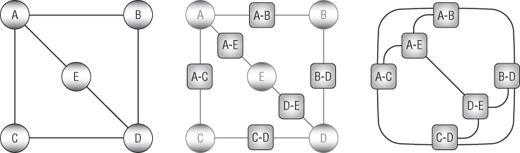
Figure 13.24: You can use an interchange network to represent a network's turn penalties.
The next step is to connect two new nodes if their corresponding original links share a common node in the original network. You can also see that connection in the new nodes' names. For example, new nodes A-B and B-D both have B in their names because their corresponding links in the original network share node B. That means the new nodes should be connected with a link in the interchange network.
That new link represents a turn in the original network starting at node A, moving to node B, and then turning to node D. You could name that link A-B-D to make the turn more obvious.
The picture on the right in Figure 13.24 shows the completed interchange network. The A-B-D link is the one in the upper-right corner of the final network.
Now instead of finding a shortest path tree in the original network, you can find one in the interchange network. When you visit a node, you add that node's cost, which corresponds to a link's cost in the original network. When you cross a link, you add that link's cost, which represents a turn penalty in the original network.
Summary
Many of the algorithms described in this chapter are traversals of networks. The depth-first and breadth-first traversal algorithms visit a network's nodes in different orders. The connectivity, spanning tree, minimal spanning tree, and shortest path algorithms also all traverse the network in various ways. For example, the minimal spanning tree algorithm traverses links in order of their costs, and the label-setting shortest path algorithm traverses links in order of the distances between each node and the root.
The next chapter continues the discussion of networks. It explains more-advanced algorithms that let you solve real-world problems such as task ordering, map coloring, and work assignment.
Exercises
You can find the answers to these exercises in Appendix B. Asterisks indicate particularly difficult problems.
- *Build a program similar to the one shown in Figure 13.25 that lets you construct, save, and load test networks. The first few tools on the toolbar should let the user add nodes, one-way links, and two-way links (or two links connecting the clicked nodes in both directions). Give the File menu the commands New, Open, and Save As to let the user create, load, and save networks. (If you're using C# or Python and don't want to build the whole program, you can download the example program from this book's website and replace the algorithmic code that it contains with your own code.)
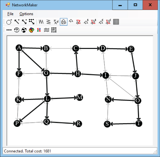
Figure 13.25: The sample program NetworkMaker lets you build, save, and load test networks.
- Expand the program you wrote for the preceding exercise to let the user perform either a depth-first or breadth-first traversal of the network. If the user selects a traversal tool and then clicks a node, display the appropriate traversal.
- Expand the program you wrote for the preceding exercise to add a tool that displays the network's connected components.
- Does the algorithm described for finding a network's connected components work for directed networks? Why or why not?
- Expand the program you wrote for Exercise 3 to add a tool that finds and displays a spanning tree rooted at a node the user clicks.
- Can you think of a simple feature of a network that would mean that all of its possible spanning trees are minimal?
- Expand the program you wrote for Exercise 5 to add a tool that finds and displays a minimal spanning tree rooted at a node the user clicks.
- Expand the program you wrote for the preceding exercise to add a tool that uses a spanning tree to find and display a path between two nodes the user selects.
- Is a shortest path tree always a minimal spanning tree? If so, why? If not, draw a counterexample.
- Expand the program you wrote for Exercise 8 to add a tool that finds and displays a label-setting shortest path tree rooted at a node the user clicks.
- Expand the program you wrote for the preceding exercise to add a tool that uses a label-setting shortest path tree to find and display a path between two nodes the user selects.
- Expand the program you wrote for the preceding exercise to add a tool that finds and displays a label-correcting shortest path tree rooted at a node the user clicks.
- Expand the program you wrote for the preceding exercise to add a tool that uses a label-correcting shortest path tree to find and display a path between two nodes the user selects.
- What happens to the label-correcting shortest path algorithm if the network contains a cycle that has a negative total weight? What happens to the label-setting algorithm?
- Suppose that you want to find the shortest path from your location to a relatively close donut shop in a large street network. How could you make a label-setting algorithm find the path without building the entire shortest path tree? Would the change save time?
- *For the scenario in the preceding exercise, how could you make a label-correcting algorithm find the path without building the entire shortest path tree? Would the change save time?
- *Suppose that you're driving to a museum and frequent road construction makes you leave the shortest path. After each change, you need to calculate a new shortest path tree to find the best route from your new location to the museum. How could you avoid those recalculations?
- *Expand the program you wrote for Exercise 13 to add a tool that finds and displays the
DistanceandViaarrays for a network. Verify the program on a network similar to the one shown in Figure 13.16. - *Expand the program you wrote for the preceding exercise so that the all-pairs shortest path tool uses text output to display the shortest paths between every pair of nodes in the network. Verify the program on a network similar to the one shown in Figure 13.16.
- Assuming that your computer can execute 1 million steps per second while building the all-pairs shortest path algorithm's
DistanceandViaarrays, how long would it take to build the arrays for a network with 100 nodes? 1,000 nodes? 10,000 nodes? - Using the network shown in Figure 13.26, draw the
DistanceandViaarrays as they evolve the same way as Figure 13.16 does. What are the initial and final shortest paths from node A to node C?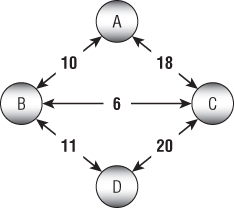
Figure 13.26: Draw the
DistanceandViaarrays for this network. - The section “Depth-First Traversal” in this chapter said that when executed on a network containing N nodes, a simple recursive traversal algorithm might reach a recursive depth of N. Can you think of networks structures for which that happens no matter which node you pick as a starting node?
- The discussion on general transitive reductions converted a network into a condensation where condensed nodes represented the original network's strongly connected components. The discussion then mentioned that the resulting condensed network was acyclic. Why is that true?
- In Figure 13.21, how many nodes and links would the network contain if it represented every dot separately? How many would it contain if it represents the connectivity and shape information separately?
- How many links in total would be required to represent completely every turn in the expanded node shown in Figure 13.23? Draw the fully expanded node.