CHAPTER 14
More Network Algorithms
Chapter 13 focused on network traversal algorithms, including algorithms that use breadth-first and depth-first traversals to find the shortest paths between nodes in the network. This chapter continues the discussion of network algorithms. The first algorithms, which perform topological sorting and cycle detection, are relatively simple. The algorithms described later in the chapter, such as graph coloring and maximal flow calculation, are a bit more challenging.
Topological Sorting
Suppose that you want to perform a complicated job that involves many tasks, some of which must be performed before others. For example, suppose you want to remodel your kitchen. Before you can get started, you may need to obtain permits from your local government. Then you need to order new appliances. Before you can install the appliances, however, you need to make any necessary changes to the kitchen's wiring. That may require demolishing the walls, changing the wiring, and then rebuilding the walls. A complex project such as remodeling an entire house or commercial building might involve hundreds of steps with a complicated set of dependencies.
Table 14.1 shows some of the dependencies that you might have while remodeling a kitchen.
Table 14.1: Kitchen Remodeling Task Dependencies
| TASK | PREREQUISITE |
| Obtain permit | — |
| Buy appliances | — |
| Install appliances | Buy appliances |
| Demolition | Obtain permit |
| Wiring | Demolition |
| Drywall | Wiring |
| Plumbing | Demolition |
| Initial inspection | Wiring |
| Initial inspection | Plumbing |
| Drywall | Plumbing |
| Drywall | Initial inspection |
| Paint walls | Drywall |
| Paint ceiling | Drywall |
| Install flooring | Paint walls |
| Install flooring | Paint ceiling |
| Final inspection | Install flooring |
| Tile backsplash | Drywall |
| Install lights | Paint ceiling |
| Final inspection | Install lights |
| Install cabinets | Install flooring |
| Final inspection | Install cabinets |
| Install countertop | Install cabinets |
| Final inspection | Install countertop |
| Install flooring | Drywall |
| Install appliances | Install flooring |
| Final inspection | Install appliances |
You can represent the job's tasks as a network in which a link points from task A to task B if task B must be performed before task A. Figure 14.1 shows a network that represents the tasks listed in Table 14.1.

Figure 14.1: You can represent a series of partially-ordered tasks as a network.
A partial ordering is a set of dependencies that defines an ordering relationship for some but not necessarily all of the objects in a set. The dependencies listed in Table 14.1 and shown in Figure 14.1 define a partial ordering for the remodeling tasks.
If you actually want to perform the tasks, you need to extend the partial ordering to a complete ordering so that you can perform the tasks in a valid order. For example, the conditions listed in Table 14.1 don't explicitly prohibit you from installing the flooring before you do the plumbing work, but if you carefully study the table or the network, you'll see that you can't do those tasks in that order. The flooring must come after painting the walls, which must come after drywall, which must come after plumbing.
Topological sorting is the process of extending a partial ordering to a full ordering on a network.
One algorithm for extending a partial ordering is quite simple. If the tasks can be completed in any valid order, then there must be some task with no prerequisites that you can perform first. Find that task, add it to the extended ordering, and remove it from the network. Then repeat those steps, finding another task with no prerequisites, adding it to the extended ordering, and removing it from the network until all of the tasks have been completed.
If you reach a point where every remaining task has a prerequisite, then the tasks have a circular dependency so that the partial ordering cannot be extended to a full ordering.
The following pseudocode shows the basic algorithm:
// Return the nodes completely ordered.List(Of Node) ExtendPartialOrdering()// Make the list of nodes in the complete ordering.List(Of Node): orderingWhile <the network contains nodes>// Find a node with no prerequisites.Node: ready_nodeready_node = <a node with no prerequisites>If <ready_node == null> Then Return null// Move the node to the result list.<Add ready_node to the ordering list><Remove ready_node from the network>End WhileReturn orderingEnd ExtendPartialOrdering
The basic idea behind the algorithm is straightforward. The trick is implementing the algorithm efficiently. If you just look through the network at each step to find a task with no prerequisites, you might perform ![]() steps each time, for a total run time of
steps each time, for a total run time of ![]()
A better approach is to give each network node a new NumBeforeMe property that holds the number of the node's prerequisites. You start by initializing each node's NumBeforeMe value. Now when you remove a node from the network, you follow its links and decrement the NumBeforeMe property for the nodes that are dependent on the removed node. If a node's NumBeforeMe count becomes 0, it is ready to add to the extended ordering.
The following pseudocode shows the improved algorithm:
// Return the nodes completely ordered.List(Of Node) ExtendPartialOrdering()// Make the list of nodes in the complete ordering.List(Of Node): ordering// Make a list of nodes with no prerequisites.List(Of Node): ready// Initialize.<Initialize each node's NumBeforeMe count><Add nodes with no prerequisites to the ready list>While <the ready list contains nodes>// Add a node to the extended ordering.Node: ready_node = <First node in ready list><Add ready_node to the ordering list>// Update NumBeforeMe counts.For Each link In ready_node.Links// Update this node's NumBeforeMe count.link.Nodes[1].NumBeforeMe = link.Nodes[1].NumBeforeMe - 1// See if the node is now ready for output.If (link.Nodes[1].NumBeforeMe == 0) Thenready.Add(link.Nodes[1])End IfNext linkEnd WhileIf (<Any node has NumBeforeMe > 0>) Then Return nullReturn orderingEnd ExtendPartialOrdering
This algorithm assumes that the network is completely connected. If it is not, use the algorithm repeatedly for each connected component.
Cycle Detection
Cycle detection is the process of determining whether a network contains a cycle. In other words, it is the process of determining whether there is a path through the network that returns to its beginning.
Cycle detection is easy if you think of the problem as one of topological sorting. A network contains a cycle if and only if it cannot be topologically sorted. In other words, if you think of the network as a topological sorting problem, then the network contains a cycle if a series of tasks A, B, C, …, K forms a dependency loop.
After you make that observation, detecting cycles is easy. The following pseudocode shows the algorithm:
// Return True if the network contains a cycle.Boolean: ContainsCycle()// Try to topologically sort the network.If (ExtendPartialOrdering() == null) Then Return TrueReturn FalseEnd ContainsCycle
This algorithm assumes that the network is completely connected. If it is not, use the algorithm repeatedly for each connected component.
Map Coloring
In map coloring, the goal is to color the regions in a map so that no regions that share an edge have the same color. Obviously, you can do this if you give every region a different color. The real question is, “What is the smallest number of colors that you can use to color a particular map?” A related question is, “What is the smallest number of colors that you can use to color any map?”
To study map coloring with network algorithms, you need to convert the problem from one of coloring regions into one of coloring nodes. Simply create a node for each region, and make an undirected link between two nodes if their corresponding regions share a border.
Depending on the map, you may be able to color it with two, three, or four colors. The following sections describe these maps and algorithms that you can use to color them.
Two-Coloring
Some maps, such as the one shown in Figure 14.2, can be colored with only two colors.

Figure 14.2: Some maps can be colored with only two colors.

Figure 14.3: If you draw a closed curve without lifting the pencil and without making any “doubled edges,” the result is two-colorable.
Coloring this kind of map is easy. Pick any region and give it one of the two colors. Then give each of its neighbors the other color, and recursively visit them to color their neighbors. If you ever come to a point where a node's neighbor already has the same color as the node, the map cannot be two-colored.
The following pseudocode shows this algorithm:
TwoColor()// Make a queue of nodes that have been colored.Queue(Of Node): colored// Color the first node, and add it to the list.Node: first_node = <Any node>first_node.Color = color1colored.Enqueue(first_node)// Traverse the network, coloring the nodes.While (colored contains nodes)// Get the next node from the colored list.Node: node = colored.Dequeue()// Calculate the node's neighbor color.Color: neighbor_color = color1If (node.Color == color1) Then neighbor_color = color2// Color the node's neighbors.For Each link In node.LinksNode: neighbor = link.Nodes[1]// See if the neighbor is already colored.If (neighbor.Color == node.Color) Then<The map cannot be two-colored>Else If (neighbor.Color == neighbor_color) Then// The neighbor has already been colored correctly.// Do nothing else.Else// The neighbor has not been colored. Color it now.neighbor.Color = neighbor_colorcolored.Enqueue(neighbor)End IfNext linkEnd WhileEnd TwoColor
This algorithm assumes that the network is completely connected. If it is not, use the algorithm repeatedly for each connected component.
Three-Coloring
It turns out that determining whether a map is three-colorable is a difficult problem. In fact, no known algorithm can solve this problem in polynomial time.
One fairly obvious approach is to try each of the three colors for the nodes and see whether any combination works. If the network holds N nodes, then this takes ![]() time, which is quite slow if N is large. You can use a tree traversal algorithm, such as one of the decision tree algorithms described in Chapter 12, to try combinations, but this still will be a very slow search.
time, which is quite slow if N is large. You can use a tree traversal algorithm, such as one of the decision tree algorithms described in Chapter 12, to try combinations, but this still will be a very slow search.
You may be able to improve the search by simplifying the network. If a node has fewer than three neighbors, then those neighbors can use at most two of the available colors, so the original node can use one of the unused colors. In that case, you can remove the node with fewer than three neighbors from the network, color the smaller network, and then restore the removed node, giving it a color that isn't used by a neighbor.
Removing a node from the network reduces the number of neighbors for the remaining nodes, so you might be able to remove even more nodes. If you're lucky, the network will shrink until you're left with a single node. You can color that node and then add the other nodes back into the network, one at a time, coloring each in turn.
The following steps describe an algorithm that uses this approach:
- Repeat while the network has a node with degree less than 3:
- Remove a node with degree less than 3, keeping track of where the node was so that you can restore it later.
- Use a network traversal algorithm to find a three-coloring for whatever network remains. If there is no solution for the smaller network, then there is no solution for the original network.
- Restore the nodes removed earlier in last-removed, first-restored order, and color them using colors that are not already used by their neighbors.
If the network is not completely connected, you can use the algorithm for each of its connected components.
Four-Coloring
The four-coloring theorem states that any map can be colored with at most four colors. This theorem was first proposed by Francis Guthrie in 1852 and was studied extensively for 124 years before Kenneth Appel and Wolfgang Haken finally proved it in 1976. Unfortunately, their proof exhaustively examined a set of 1,936 specially selected maps, so it doesn't offer a good method of finding a four-coloring of a map.
You can use techniques similar to those described in the previous section for three-coloring.
- Repeat while the network has a node with degree less than 4:
- Remove a node with degree less than 4, keeping track of where the node was so that you can restore it later.
- Use a network traversal algorithm to find a four-coloring for whatever network remains. If there is no solution for the smaller network, then there is no solution for the original network.
- Restore the nodes removed earlier in last-removed, first-restored order, and color them using colors that are not already used by their neighbors.
Again, if the network is not completely connected, you can use the algorithm for each of its connected components.
Five-Coloring
Even though there is no simple constructive algorithm for four-coloring a map, there is an algorithm for five-coloring a map, even if it isn't very simple.
Like the algorithms described in the two previous sections, this algorithm repeatedly simplifies the network. Unlike the two previous algorithms, this one can always simplify the network until it eventually contains only a single node. You can then undo the simplifications to rebuild the original network, coloring the nodes as you go.
This algorithm uses two types of simplification. The first is similar to the one used by the two previous algorithms. If the network contains a node that has fewer than five neighbors, remove it from the network. When you restore the node, give it a color that is not used by one of its neighbors. Let's call this Rule 1.
You use the second simplification if the network doesn't contain any node with fewer than five neighbors. It can be shown (although it's outside the scope of this book) that such a network must have at least one node K with neighbors M and N such that:
- K has exactly five neighbors.
- M and N have at most seven neighbors.
- M and N are not neighbors of each other.
To simplify the network, find such nodes K, N, and M, and require that nodes M and N have the same color. We know that they aren't neighbors, so that is allowed. Because node K has exactly five neighbors and nodes M and N use the same color, K's neighbors cannot be using all five of the available colors. This means that at least one color is left over for node K.
The simplification is to remove nodes K, M, and N from the network and create a new node M/N to represent the color that nodes M and N will have. Give the new node the same neighbors that nodes M and N had previously. Let's call this Rule 2.
When you restore the nodes K, M, and N that were removed using Rule 2, give nodes M and N whatever color was assigned to node M/N. Then pick a color that isn't used by one of its neighbors for node K.
You can use techniques similar to those described in the previous section for three-coloring. The following steps describe the algorithm:
- Repeat while the network has more than one node:
- If there is a node with degree less than 5, then remove it from the network, keeping track of where it was so that you can restore it later.
- If the network contains no node of degree less than 5, then find a node K with degree exactly 5 and two children M and N, as described earlier. Replace nodes K, M, and N with new node M/N, as described in Rule 2.
- When the network contains a single node, assign it a color.
- Restore the previously removed nodes, coloring them appropriately.
If the network is not completely connected, then you can use the algorithm for each of its connected components.
Figure 14.4 shows a small sample network being simplified. If you look closely at the network on the left, you'll see that every node has five neighbors, so you can't use Rule 1 to simplify the network.

Figure 14.4: You can simplify this network to a single node with one use of Rule 2 and several uses of Rule 1.
You can't use Rule 1 on this network, but you can use Rule 2. There are several possible choices for nodes to play the roles of nodes K, M, and N in Rule 2. This example uses the nodes C, B, and H, which are drawn in bold in the network on the left. Those nodes are removed, and a new node B/H is added with the same children that nodes B and H had before. The second network in Figure 14.4 shows the revised network.
After nodes C, B, and H have been replaced with the new node B/H, nodes G, A, and D have fewer than five neighbors, so they are removed. Those nodes are highlighted in bold in the second network in Figure 14.4. For this example, assume that the nodes are removed in the order G, A, D. The third network in Figure 14.4 shows the result.
After those nodes have been removed, nodes L, B/H, K, F, E, and I all have fewer than five neighbors, so they are removed next. Those nodes are highlighted in the third network in Figure 14.4.
At this point, the network contains only the single node J, so the algorithm arbitrarily assigns node J a color and begins reassembling the network.
Suppose that the algorithm gives nodes the colors red, green, blue, yellow, and orange in that order. For example, if a node's neighbors are red, green, and orange, then the algorithm gives the node the first unused color—in this case, blue.
Starting at the final network shown in Figure 14.4, the algorithm follows these steps:
- The algorithm makes node J red.
- The algorithm restores the node that was removed last, node I. Node I's neighbor J is red, so the algorithm makes node I green.
- The algorithm restores the node that was removed next-to-last, node E. Node E's neighbors J and I are red and green, so the algorithm makes node E blue.
- The algorithm restores node F. Node F's neighbors J and E are red and blue, so the algorithm makes node F green.
- The algorithm restores node K. Node K's neighbors J and F are red and green, so the algorithm makes node K blue.
- The algorithm restores node B/H. Node B/H's neighbors K, F, and I are blue, green, and green, so the algorithm makes node B/H red.
- The algorithm restores node L. Node L's neighbors K, B/H, and I are blue, red, and green, so the algorithm makes node L yellow. (At this point, the network looks like the bottom network in Figure 14.4, but with the nodes colored.)
- The algorithm restores node D. Node D's neighbors B/H, E, and I are red, blue, and green, so the algorithm makes node D yellow.
- The algorithm restores node A. Node A's neighbors B/H, F, E, and D are red, green, blue, and yellow, so the algorithm makes node A orange.
- The algorithm restores node G. Node G's neighbors L, B/H, and K are yellow, red, and blue, so the algorithm makes node G green. (At this point the network looks like the middle network in Figure 14.4, but with the nodes colored.)
- Now the algorithm undoes the Rule 2 step. It restores nodes B and H and gives them the same color as node B/H, which is red. Finally, it restores node C. Its neighbors G, H, D, A, and B have colors green, red, yellow, orange, and red, so the algorithm makes node C blue.
At this point, the network looks like the original network on the left in Figure 14.4 but colored as shown in Figure 14.5. (The figure uses shades of gray because this book isn't printed in color.)

Figure 14.5: This network is five-colored.
Other Map-Coloring Algorithms
These are not the only possible map-coloring algorithms. For example, a hill-climbing strategy might loop through the network's nodes and give each one the first color that is not already used by one of its neighbors. This may not always color the network with the fewest possible colors, but it is extremely simple and very fast. It also works if the network is not planar and it might be impossible to four-color the network. For example, this algorithm can color the non-planar network shown in Figure 14.6.

Figure 14.6: This network is not planar, but it can be three-colored.
With some effort, you could apply some of the other heuristic techniques described in Chapter 12 to try to find the smallest number of colors needed to color a particular planar or nonplanar network. For example, you could try random assignments or incremental improvement strategies in which you switch the colors of two or more nodes. You might even be able to create some interesting swarm intelligence algorithms for map coloring.
Maximal Flow
In a capacitated network, each of the links has a maximum capacity indicating the maximum amount of some sort of flow that can cross it. The capacity might indicate the number of gallons per minute that can flow through a pipe, the number of cars that can move through a street per hour, or the maximum amount of current a wire can carry.
In the maximal flow problem, the goal is to assign flows to the links to maximize the total flow from a designated source node to a designated sink node.
For example, consider the networks shown in Figure 14.7. The numbers on a link show the link's flow and capacity. For example, the link between nodes B and C in the left network has a flow of 1 and a capacity of 2.

Figure 14.7: In the maximal flow problem, the goal is to maximize the flow from a source node to a sink node.
The network on the left has a total flow of 4 from node A to node F. The total amount of flow leaving the source node A in the network on the left is 1 unit along the A → D link plus 3 units along the A → B link for a total of 4. Similarly, the total flow into the sink node F is 3 units along the E → F link plus 1 unit along the C → F link for a total of 4 units. (If no flow is gained or lost in the network, then the total flow out of the sink node is the same as the total flow into the sink node.)
You cannot increase the total flow by simply adding more flow to some of the links. In this example, you can't add more flow to the A → B link because that link is already used at full capacity. You also can't add more flow to the A → D link because the E → F link is already used at full capacity, so the extra flow wouldn't have anywhere to go.
You can improve the solution, however, by removing 1 unit of flow from the path B → E → F and moving it to the path B → C → F. That gives the E → F link unused capacity so you can add a new unit of flow along the path A → D → E → F. The network on the right in Figure 14.7 shows the new flows, giving a total flow of 5 from node A to node F.
The algorithm for finding maximal flows is fairly simple, at least at a high level, but figuring out how it works can be hard. To understand the algorithm, it helps to know a bit about residual capacities, residual capacity networks, and augmenting paths.
If that sounds intimidating, don't worry. These concepts are useful for understanding the algorithm, but you don't need to build many new networks to calculate maximal flows. Residual capacities, residual capacity networks, and augmenting paths can all be found within the original network without too much extra work.
A link's residual capacity is the amount of extra flow you could add to the link. For example, the C → F link on the left in Figure 14.7 has a residual capacity of 2 because the link has a capacity of 3 and is currently carrying a flow of only 1.
In addition to the network's normal links, each link defines a virtual backlink that may not actually be part of the network. For example, in Figure 14.7, the A → B link implicitly defines a backward B → A backlink. These backlinks are important because they can have residual capacities, and you may be able to push flow backward across them.
A backlink's residual capacity is the amount of flow traveling forward across the corresponding normal link. For example, on the left in Figure 14.7, the B → E link has a flow of 2, so the E → B backlink has a residual capacity of 2. (To improve the solution on the left, the algorithm must push flow back across the E → B backlink to free up more capacity on the E → F link. That's how the algorithm uses the backlinks' residual capacities.)
A residual capacity network is a network consisting of links and backlinks marked with their residual capacities. Figure 14.8 shows the residual capacity network for the network on the left in Figure 14.7. Backlinks are drawn with dashed lines.

Figure 14.8: A residual capacity network shows the residual capacity of a network's links and backlinks.
For example, the C → F link on the left in Figure 14.7 has a capacity of 3 and a flow of 1. Its residual capacity is 2 because you could add two more units of flow to it. Its backlink's residual capacity is 1 because you could remove one unit of flow from the link. In Figure 14.8, you can see that the C → F link is marked with its residual capacity 2. The F → C backlink is marked with its residual capacity 1.
To improve a solution, all you need to do is to find a path through the residual capacity network from the source node to the sink node that uses links and backlinks with positive residual capacities. Then you push additional flow along that path. Adding flow to a normal link in the path represents adding more flow to that link in the original network. Adding flow to a backlink in the path represents removing flow from the corresponding normal link in the original network. Because the path reaches the sink node, it increases the total flow to that node. Because the path improves the solution, it is called an augmenting path.
The bold links in Figure 14.8 show an augmenting path through the residual capacity network for the network shown on the left in Figure 14.7.
To decide how much flow the path can carry, follow the path from the sink node back to the source node, and find the link or backlink with the smallest residual capacity. Now you can update the network's flows by moving that amount through the path. If you update the network on the left of Figure 14.7 by following the augmenting path in Figure 14.8, you get the network on the right in Figure 14.7.
This may seem complicated, but the algorithm isn't too confusing after you understand the terms. The following steps describe the algorithm, which is called the Ford–Fulkerson algorithm:
- Repeat as long as you can find an augmenting path through the residual capacity network:
- Find an augmenting path from the source node to the sink node.
- Follow the augmenting path, and find the smallest residual capacity along it.
- Follow the augmenting path again, and update the links' flows to push the new flow along the augmenting path.
Remember that you don't actually need to build the residual capacity network. You can use the original network and calculate each link's and backlink's residual capacity by comparing its flow to its capacity.
Network flow algorithms have several applications other than calculating actual flows such as water or current flow. The next two sections describe two of those: performing work assignment and finding minimal flow cuts.
Work Assignment
Suppose that you have a workforce of 100 employees, each with a set of specialized skills, and you have a set of 100 jobs that can only be done by people with certain combinations of skills. The work assignment problem asks you to assign employees to jobs in a way that maximizes the number of jobs that are done.
At first this might seem like a complicated combinatorial problem. You could try all of the possible assignments of employees to jobs to see which one results in the most jobs being accomplished. There are ![]() permutations of employees, so that could take a while. You might be able to apply some of the heuristics described in Chapter 12 to find approximate solutions, but there is a better way to solve this problem.
permutations of employees, so that could take a while. You might be able to apply some of the heuristics described in Chapter 12 to find approximate solutions, but there is a better way to solve this problem.
The maximal flow algorithm gives you an easy solution. Create a work assignment network with one node for each employee and one node for each job. Create a link from an employee to every job that the employee can do. Create a source node connected to every employee, and connect every job to a sink node. Give all of the links a capacity of 1.
Figure 14.9 shows a work assignment network with five employees represented by letters and five jobs represented by numbers. All of the links are directional, point to the right, and have a capacity of 1. The arrowheads and capacities are not shown to keep the picture simple.

Figure 14.9: The maximal flow through a work assignment network gives optimal assignments.
Now find the maximal flow from the source node to the sink node. Each unit of flow moves through an employee to the job that should be assigned to that employee. The total flow gives the number of jobs that can be performed.
Minimal Flow Cut
In the minimal flow cut problem (also called min flow cut, minimum cut, or min-cut), the goal is to remove links from a network to separate a source node from a sink node while minimizing the capacity of the links removed.
For example, consider the network shown in Figure 14.10. Try to find the best links to remove to separate source node A from sink node O. You could remove the A → B and A → E links, which have a combined capacity of 9. You can do better if you remove the K → O, N → O, and P → O links instead, because they have a total capacity of only 6. Take a minute to see how good a solution you can find.

Figure 14.10: Try to find the best links to remove from this network to separate node A from node O.
Exhaustively removing all possible combinations of links would be a huge task for even a relatively small network. Each link is either removed or left in the network, so if the network contains N links, there would be ![]() possible combinations of removing and leaving links. The relatively small network shown in Figure 14.10 contains 24 links, so there are 224 ≈ 16.8 million possible combinations to consider. In a network with 100 links, which is still fairly small for many applications, such as a modeling a street network, you would need to consider
possible combinations of removing and leaving links. The relatively small network shown in Figure 14.10 contains 24 links, so there are 224 ≈ 16.8 million possible combinations to consider. In a network with 100 links, which is still fairly small for many applications, such as a modeling a street network, you would need to consider ![]() combinations. If your computer could consider 1 million combinations per second, it would take roughly
combinations. If your computer could consider 1 million combinations per second, it would take roughly ![]() years to consider them all. You could undoubtedly come up with some heuristics to make the search easier, but this would be a daunting approach.
years to consider them all. You could undoubtedly come up with some heuristics to make the search easier, but this would be a daunting approach.
Fortunately, the maximal flow algorithm provides a much easier solution. The following steps describe the algorithm at a high level:
- Perform a maximal flow calculation between the source and sink nodes.
- Starting from the sink node, visit all of the nodes that you can visit using only links and backlinks that have residual capacities greater than 0.
- Place all of the nodes that you visited in step 2 in set A and place all of the other nodes in set B.
- Remove the links that lead from nodes in set A to nodes in set B.
The algorithm is relatively simple. Unfortunately, the reasons why it works are fairly confusing.
First, consider a maximal set of flows, suppose the total maximum flow is F, and consider the cut produced by the algorithm. This cut must separate the source and sink nodes. If it didn't, then there would be a path from the source to the sink through which you could move more flow. In that case, there would be a corresponding augmenting path through the residual capacity network, so the maximal flow algorithm executed in step 1 would not have done its job correctly.
Notice that any cut that prevents flow from the source node to the sink node must have a net flow of F across its links. Flow might move back and forth across the cut, but in the end F units of flow reach the sink node, so the net flow across the cut is F.
This means that the links in the cut produced by the algorithm must have a total capacity of at least F. All that remains is to see why those links have a total capacity of only F. The net flow across the cut is F, but perhaps some of the flow moves back and forth across the cut, increasing the total flow of the cut's links.
Suppose this is the case, so a link L flows back from the nodes in set B to the nodes in set A and then later another link moves the flow back from set A to set B. The flow moving across the cut from set B to set A and back from set A to set B would cancel, and the net result would be 0.
If there is such a link L, however, it has positive flow from set B to set A. In that case, its backlink has a positive residual capacity. But in step 2, the algorithm followed all links and backlinks with positive residual capacity to create set A. Because link L ends at a node in set A and has positive residual capacity, the algorithm should have followed it, and the node at the other end should also have been in set A.
All of this means that there can be no link from set B to set A with positive flow.
Because the net flow across the cut is F and there can be no flow backward across the cut into the nodes in set A, the flow across the cut must be exactly F, and the total capacity removed by the cut is F.
(I warned you that this would be confusing. The technical explanation used by graph theorists is even more confusing.)
Now that you've had time to work on the problem shown in Figure 14.10, here's the solution. The optimal cut is to remove links E → I, F → J, F → G, C → G, and C → D, which have a total capacity of 4. Figure 14.11 shows the network with those links removed.

Figure 14.11: This network shows a solution to the min-flow-cut problem for the network shown in Figure 14.10.
Note that the solution to the minimal flow cut problem may not be unique. For example, the links M → N, J → N, K → O, and P → O also have a total cost of 4, and removing them from the network shown in Figure 14.10 also separates nodes A and O.
Network Cloning
Suppose that you want to make a clone of an existing network. A traversal algorithm, such as those described earlier in this chapter, lets you visit the nodes in the network. You could traverse the network and make copies of its nodes, but that wouldn't connect the copied nodes with links that mimic the links in the original network.
After you clone the network's nodes, you need to connect them with appropriate links. To clone a link, you need to find the two cloned nodes that correspond to the link's nodes in the original network.
The following sections explain two simple ways that you can find those nodes so that you can clone the link. Both of these methods assume that you have a list or array containing references to all of the original network's nodes. You can use a traversal to build that list if you don't already have one.
Dictionaries
One way to find the new nodes that correspond to a link's original nodes is to use a dictionary. When you clone a node, store the new node in the dictionary and use the original node as its key. Then you can use the original node later to look up the cloned version.
The following pseudocode shows how you can use this approach to clone a network:
// Clone a network.Node[]: CloneNetwork(Node[]: nodes)// Make a dictionary to hold the new nodes.Dictionary<Node, Node>: nodeDict = New Dictionary<Node, Node>()// Clone the nodes.Node[]: newNodes = new Node[nodes.Length]For i = 0 To nodes.Length -1Node: oldNode = nodes[i]Node: newNode = <Clone of oldNode>newNodes[i] = newNodenodeDict.Add(oldNode, newNode)Next i// Clone the links.For i = 0 To nodes.Length - 1Node: oldNode = nodes[i]Node: newNode = newNodes[i]For Each link In oldNode.LinksNode: newNeighbor = nodeDict[link.Neighbor]<Add link between newNode and newNeighbor>Next neighborNext ireturn newNodesEnd CloneNetwork
The algorithm first creates a dictionary that uses Node objects as both keys and data values. Next, it creates an array to hold the cloned nodes. It then loops through the existing nodes and places clones of them in the new array. It also places the cloned nodes in the dictionary using their original nodes as keys.
After it finishes cloning the nodes, the algorithm loops through the original nodes again and loops through each original node's links. For each link, it finds the node's neighbor at the other end of the link. It then uses the dictionary to find the neighbor's clone. Finally, it makes a new link between the node's clone and the neighbor's clone.
The exact details of how you clone a node depend on the way you are storing the network. When you clone the node, you need to copy any important details from the old node into the clone. For example, you might need to copy the node's name, location, colors, or other attributes.
Similarly, the way that you clone the link depends on how you store links. For example, if a node directly stores references to its neighboring nodes in a list, then you need to add references to the cloned neighbors to the cloned node's list. In contrast, if a node's links are stored in separate Link objects, then you need to make a new cloned Link object, copy any important properties such as cost or capacity into the clone, and set the clone's Node objects to the cloned node and the cloned neighbor.
Clone References
The trickiest part of network cloning is figuring out which cloned node belongs at the end of a cloned link. The algorithm described in the preceding section uses a dictionary to map original nodes to cloned nodes, but there are other options. For example, you could add a new ClonedNode field to the Node class. Then when you clone a node, you can save a reference to the clone inside the original node for later reference.
In fact, that approach is more efficient than using a dictionary because it stores only a single clone reference per node, and it allows you to find a node's clone immediately. In contrast, a dictionary requires a more complicated data structure such as linked lists or a hash table. Those data structures take up additional space and require extra steps to save and retrieve values.
The following pseudocode shows how you could modify the previous algorithm to use a ClonedNode field. The modified code is highlighted in bold.
// Clone a network.Node[]: CloneNetwork(Node[]: nodes)// Clone the nodes.Node[]: newNodes = new Node[nodes.Length]For i = 0 To nodes.Length -1Node: oldNode = nodes[i]Node: newNode = <Clone of oldNode>newNodes[i] = newNodeoldNode.ClonedNode = newNodeNext i// Clone the links.For i = 0 To nodes.Length - 1Node: oldNode = nodes[i]Node: newNode = newNodes[i]For Each link In oldNode.LinksNode: newNeighbor = link.Neighbor.ClonedNode<Add link between newNode and newNeighbor>Next neighborNext ireturn newNodesEnd CloneNetwork
Instead of storing a cloned node in a dictionary, this version simply stores each node's clone in its ClonedNode field. Then it can easily find the node's clone when it needs it later.
An alternative to storing the clone in a node is to store the index of the clone in the newNodes array. Then you can use the index to retrieve the clone whenever you need it.
Cliques
A clique is a subset of nodes within an undirected graph that are all mutually connected. A k-clique is a clique that contains k nodes. A maximal clique is a clique that cannot be extended without ruining its clique-ness.
Figure 14.12 shows a small network with two maximal cliques circled in dashed lines. One clique includes the nodes { A, B, D }, and the other includes nodes { B, C, D, E }. Both are maximal cliques because they are as large as possible while still being cliques.

Figure 14.12: A clique is a subset of mutually connected nodes.
There are many different types of clique problems including the following:
- Find a maximum clique (the largest clique in the graph).
- List all maximal cliques (cliques that cannot be enlarged).
- Find a maximum weight clique (with the largest total edge weight).
- Determine whether there is a clique of size K.
For example, { B, C, D, E } is the maximum clique in the graph shown in Figure 14.12 because there are no larger cliques. The clique { A, B, D } is maximal because you cannot add another node to it while keeping all of the nodes mutually connected.
Note that every node forms a single-node clique and any pair of nodes that are connected by a link form a two-node clique.
The following sections describe some algorithms that solve particular clique problems.
Brute Force
A brute-force approach is rarely the best way to attack a problem, but at least it is usually easy to understand. One way to find a clique containing K nodes would be to enumerate every possible selection of K nodes and then check them to see whether they form a clique. If the network contains N nodes, then the number of possible selections is given by the binomial coefficient, which is calculated by the following equation:

For example, if the network contains 10 nodes, then the number of ways that you can select four nodes is the following:

This means you need to check up to 210 selections of four nodes to find four-node cliques.
To see whether a clique is maximal, you can loop through the network's remaining nodes and see whether the selection is still a clique if you add each node to it. If the selection is still a clique after you add one of the remaining nodes, then it is not maximal.
To list all of a network's cliques, you can loop through all of the combinations that include 1 node, 2 nodes, 3 nodes, and so on, and see which combinations are cliques. (If you think that would be a lot of work, you're right!)
To list all of a network's maximal cliques, you can list the cliques and then test each to see whether it is maximal. (The next section describes a better method to do this.)
To find a network's largest clique, simply try to find cliques of sizes 1, 2, 3, and so on, until you find a size for which there is no clique. If a clique contains K nodes, then any subset of ![]() of those nodes is also a clique. That means if there is no clique containing M nodes, then there is no clique containing more than M nodes either.
of those nodes is also a clique. That means if there is no clique containing M nodes, then there is no clique containing more than M nodes either.
All of these methods work and are relatively straightforward, but they are also quite inefficient. The next section describes a better algorithm for performing one of those tasks: finding all of a network's maximal cliques.
Bron–Kerbosch
The Bron–Kerbosch algorithm was described by Dutch computer scientists Coenraad Bron and Joep Kerbosch in 1973. It's a recursive backtracking algorithm with a relatively simple idea.
At the very highest level, the algorithm starts with a clique and then tries to grow it by adding other nodes to it. When the clique cannot grow any larger, it is maximal, so the algorithm reports it.
If the algorithm adds a node to the clique that breaks the clique property, the algorithm backtracks to the point before that node was added.
The clever part of the algorithm is the bookkeeping that it uses to expand the cliques efficiently. The details are a bit tricky, so I'll describe them in several sections.
Sets R, P, and X
The algorithm keeps track of the network's nodes in three sets called R, P, and X.
Set R contains nodes that are in the current clique. Set P contains prospective nodes that we will try adding to the clique.
Set X contains nodes that are excluded from consideration because we have already tried using them and reported any maximal cliques that contain the nodes in R plus the nodes in X. In other words, if x is a node in X and there is a maximal clique containing ![]() , then we have already reported it. (This is probably the most confusing part of the algorithm, so be sure you understand it.)
, then we have already reported it. (This is probably the most confusing part of the algorithm, so be sure you understand it.)
An important feature of the three sets is that any node that is connected to all of the nodes in R is in one of the three sets. In particular, if node n is not currently in R and n is connected to every node in R, then it is either in P (so we will later try adding it to R) or it is in X (so we have already reported the cliques contain R and n).
Initially R is empty, so the initial clique contains no nodes. Note that you can think of an empty set (or a set that contains a single node) as a clique because it includes a path between every pair of nodes that it contains and there are no such pairs.
Set P begins holding every node in the network. In other words, every node is a candidate to add to the initially empty clique.
Set X begins empty because we haven't tried and discarded any nodes yet.
After the initialization, the algorithm checks sets P and R. If both P and R are empty, then there are no more nodes that we can add to the clique, so it is maximal.
If P is empty but X is not, then there are no more nodes that we can add to the clique. However, because X is not empty, there are cliques that contain the nodes in R and nodes in X. Those cliques are bigger than R (and we have already reported them), so the current clique is not maximal.
Recursive Calls
Now that you understand the three sets R, P, and X, you need to learn how the algorithm calls itself recursively.
Suppose that you have built a clique R. The nodes in P are candidates for expanding the clique, so you loop through those nodes and try adding each to R.
When we add a new node n to R, we should update P so it includes only nodes that we might want to add to the new clique R + n. If node q is in P and it is not a neighbor of node n, then it cannot be used to enlarge the clique further, so we should remove it from P.
We should also update X so that it doesn't include any nodes that we won't consider adding to the clique. If node q is not a neighbor of node n, then it can no longer be in P because we removed node n's non-neighbors. In that case, we don't need to exclude node q by keeping it in set X, so we can remove it.
Pseudocode
The following pseudocode shows the Bron–Kerbosch algorithm:
List Of (Set Of Node): BronKerbosch(R, P, X)cliques = New Set()If (P is empty) And (X is empty) Then cliques.Add(R)For Each n In PNew_R = R + nNew_P = P ∩ Neighbors(n)New_X = X ∩ Neighbors(n)cliques.AddRange(BronKerbosch(new_R, new_P, new_X))P = P – nX = X + nNext nodereturn cliques
The algorithm returns a list of cliques, each of which is a set of nodes.
The method starts by creating an empty cliques list to hold any maximal cliques that it finds.
Next, if the sets P and X are both empty, the method adds R to the list of maximal cliques.
The algorithm then loops through the nodes n in P and tries adding them one at a time to R. To do that, it creates updated versions of the three sets. It adds the node n to R to extend the clique. Then also takes the intersection of sets P and X with the neighbors of node n.
The code then calls the BronKerbosch method recursively, passing it the new sets.
After the recursive call returns, the code removes node n from P so that future recursive calls will not include it in the set new_P and thus will not include it in future cliques that contain the nodes in R. It also adds node n to set X so that the algorithm will not report any more cliques that contain the nodes in R plus node n.
After the algorithm has processed all of the nodes in P, it returns the maximal cliques that it found.
Example
The Bron–Kerbosch algorithm is remarkably short, but it's also pretty confusing. To make it easier to understand, let's work through an example. Consider the network shown in Figure 14.13.

Figure 14.13: You can use the Bron–Kerbosch algorithm to find this network's maximal cliques.
The example is somewhat long even though the network is small, but you should be able to follow it if you work through it slowly and carefully.
The following pseudocode shows the first call to the algorithm:
BronKerbosch({ }, {A, B, C, D}, { }) // Level 1 The sets P and X are not both empty, so the algorithm loops through the nodes in P.
The order in which items are visited in a set are not clearly defined in most programming languages because a set implies membership but not an ordering. This means that the algorithm will not necessarily visit the nodes in any particular order. For this example, let's assume that the program first visits node A.
To update the sets, the algorithm adds node A to set R and removes the non-neighbors of node A from sets P and X. That means new_R = {A}, new_P = {B, C}, and new_X = { }. The following pseudocode shows the second call to the algorithm:
BronKerbosch({A}, {B, C}, { }) // Level 2 Sets P and X are still not both empty, so the algorithm loops through the nodes in P. Let's suppose the algorithm tries node B first. It creates the sets new_R = {A, B}, new_P = {C}, and new_X = { }. The algorithm then makes the following call:
BronKerbosch({A, B}, {C}, { }) // Level 3 Sets P and X are still not both empty, so the algorithm calls itself one more time, as shown in the following pseudocode:
BronKerbosch({A, B, C}, { }, { }) // Level 4 This time P and X are both empty, so R = {A, B, C} is a maximal clique. This call to the algorithm returns that clique and then moves one step back up the call stack to level 3, which was called by the following:
BronKerbosch({A, B}, {C}, { }) // Level 3 There are no more nodes in P to loop through, so this call returns to the level 2 call:
BronKerbosch({A}, {B, C}, { }) // Level 2 The recursive call just tried adding node B to the clique. When the recursive call returns, the level 2 call removes node B from P and adds it to X. Now P = {C} and X = {B}.
This is one of the more confusing parts of the example. Each time a recursive call returns, the calling method updates its sets P and X. However, that method is still looping through the nodes that were originally in its set P. For example, set P in the level 2 call original was {B, C}. After returning from the first recursive call, the code sets P = {C}, but it still needs to loop over the remaining node in the original set, which is node C.
In this case, that means the method tries adding node C to the clique. It creates the new sets new_R = {A, C}, new_P = { }, and new_X = {B}. It then makes the following recursive call:
BronKerbosch({A, C}, { }, {B}) // Level 3 This time P is empty, but X is not. The set X contains node B indicating that we have already reported any maximal cliques that contain the nodes in R plus node B. We did report the set {A, B, C} earlier, so that is correct. This recursive call returns without doing anything interesting. It also returns the earlier level 2 call, so we arrive back at level 1, which we reached through the following call:
BronKerbosch({ }, {A, B, C, D}, { }) // Level 1 We just tried adding node A to the clique, so the algorithm updates P and X by moving node A from P and to X. Now P = {B, C, D} and X = {A}.
The algorithm then tries adding node B to the clique. To do that, it adds node B to R to get new_R = {B}. It also removes the non-neighbors of node B from P and X to get new_P = {C, D} and new_X = {A}. It then makes the following recursive call:
BronKerbosch({B}, {C, D}, {A}) // Level 2 Suppose that this call visits node C first. In that case, it adds C to R and removes non-neighbors of C from P and X. That means new_R = {B, C}, new_P = { }, and new_X = {A}. It then makes the following call:
BronKerbosch({B, C}, { }, {A}) // Level 3 This time P is empty, but X contains node A, indicating that we have already reported any maximal cliques that contain nodes {B, C} plus node {A}. The algorithm again returns without doing anything interesting.
The level 2 call moves node C from P to X and then visits node D. It adds D to R and removes non-neighbors of D from P and X to get the new sets new_P = { } and new_X = { }. It then makes the following call:
BronKerbosch({B, D}, { }, { }) // Level 3 Because sets P and X are both empty, the algorithm reports {B, D} as another maximal clique and returns. (You may not have realized that {B, D} was a maximal clique when you first saw Figure 12.14, but it is.)
The level 2 call has finished visiting the nodes in its original set P (which were C and D), so it returns to the next higher level, which we reached from this call:
BronKerbosch({ }, {A, B, C, D}, { }) // Level 1 We just tried adding node B to set R, so the algorithm updates P and X by moving B from P to X. Now R = { }, P = {C, D}, and X = {A, B}.
The method must now call itself with the next node in its original set P, which is node C. To do that, it adds node C to set R and removes the non-neighbors of node C from P and X to give new_R = {C}, new_P = { }, and new_X = {A, B}. It then makes the following call:
BronKerbosch({C}, { }, {A, B}) // Level 2 Set P is empty, but set X is not, so the method returns without doing anything interesting, and we return again to level 1:
BronKerbosch({ }, {A, B, C, D}, { }) // Level 1 We just tried adding node C to the clique. The algorithm updates its sets by moving C from set P and to set X, so P = {D} and X = {A, B, C}.
The method must now call itself with the next node in its original set P, which is node D. To do that, it adds node D to set R and removes the non-neighbors of node D from P and X to give P = { } and X = {B}. It then makes the following call:
BronKerbosch({D}, { }, {B}) // Level 2 Again, set P is empty but set X is not, so the method returns without doing anything, and we return once more to the following call:
BronKerbosch({ }, {A, B, C, D}, { }) // Level 1 We have finished looping over the nodes in the original set P, so this call returns the cliques that it has found and we are done.
The final results include the two maximal cliques {A, B, C} and {B, D}.
Variations
The Bron–Kerbosch algorithm is a big improvement over a brute-force search, but it can still give poor performance for networks that contain many non-maximal cliques. The algorithm calls itself recursively for every clique, so if the network contains many non-maximal cliques, it wastes a lot of time.
There are a couple of modified versions of the algorithm that reduce the number of nodes that must be considered in the set P. You can find descriptions of those variations on the Internet. For example, look at the following URLs:
- Wikipedia:
https://en.wikipedia.org/wiki/Bron%E2%80%93Kerbosch_algorithm - University of Glasgow:
http://www.dcs.gla.ac.uk/~pat/jchoco/clique/enumeration/report.pdf - Inria Sophia Antipolis:
ftp://ftp-sop.inria.fr/geometrica/fcazals/papers/ncliques.pdf
Finding Triangles
The previous few sections explained ways to find different kinds of cliques. One particularly simple but interesting type of clique is a triangle. The following sections describe three methods for finding a network's triangles.
Brute Force
An obvious way to find a network's triangles is to use a brute-force approach. Simply enumerate all of the possible triples of nodes and see whether they form a triangle.
One disadvantage to this method is that it considers triples of nodes that might have no chance of forming a triangle. For example, consider a street network. The brute-force approach would check whether nodes at the extreme left, right, and top edges of the network form a triangle, even though that's obviously impossible. This method will spend a lot of time checking triples of nodes that could not possibly form a triangle in any network that has relatively few links compared to the number of nodes.
Checking Local Links
One way to avoid examining triples of nodes that are far apart is to look more locally at each node's neighborhood. Starting at a selected node, you can follow its links to its neighbors. You can then see which neighbors are connected to each other. (You already know that they are connected to the original node because they are its neighbors.)
Even that approach could be confusing as you examine all of the possible pairs of neighbors. A handy way to keep track of the possible pairs is to loop through the neighbors and mark them. Next, loop through each of the neighbors' neighbors. If you find a node that is marked, then you know that the marked node is reachable from one of the other neighbors, so it makes a triangle.
For a more specific example, suppose nodes A, B, and C form a triangle. First, you mark A's neighbors, which includes nodes B and C. Next, you loop through node B's neighbors. When you do that, you will find node C and notice that it already marked. That means the original node, A; the neighbor B; and its neighbor C form a triangle.
All of this leads to the following algorithm for finding a network's triangles:
For Each node In AllNodes:// Mark the neighbors.For Each neighbor In node.Neighborsneighbor.Marked = TrueNext neighbor// Search for triangles.For Each nbr In node.Neighbors:// Search for the third node in the triangle.For Each nbr_nbr In nbr.Neighbors:If nbr.Marked Then <{node, nbr, nbr_nbr} is a triangle.>Next nbrNext nbr// Unmark the neighbors.For Each neighbor In node.Neighborsneighbor.Marked = FalseNext neighborNext node
This algorithm works and doesn't waste time examining widely spaced triples, but it does have one other problem. When you loop through node A's neighbors, you will first find node B and then later you will find node C. This means that you will find, the triangle {A, B, C} and then later the same triangle {A C, B}.
Worse still, you will later use node B as the starting node, so you'll also find triangles {B, A, C} and {B, C, A}. Then when you use node C as a starting node, you'll find triangles {C, A, B} and {C, B, A}. In total, the algorithm finds each triangle six times with different node orderings.
One way to prevent that is to compare the nodes' names, indices, or some other unique feature and only report triangles where the three nodes have a certain ordering. For example, if you compare the nodes' names, you might only report triangles where A.Name < B.Name < C.Name. If each node's name is different, then only one of the six arrangements of items will satisfy the ordering, so the algorithm will generate each triangle only once.
Chiba and Nishizeki
The algorithm described in the preceding section is actually a simplified version of an algorithm described in 1985 by Japanese computer scientists Norishige Chiba and Takao Nishizeki. Their algorithm first sorts the nodes by their degrees. It then examines the nodes in order, largest degree to smallest, and uses the preceding algorithm to find triangles.
When it examines node N, the algorithm works much as the previous one did. It marks N's neighbors and then searches the neighbors' neighbors to find triangles. After it has found all of the triangles that contain node N, it unmarks N's neighbors. It then removes N from the network. That prevents the algorithm from finding the same triangles that contain N again later. It also reduces the size of the network so N's neighbors will have fewer links to search when the algorithm encounters them again.
Of course, Chiba and Nishizeki's algorithm also destroys the network because it removes nodes from it. To avoid that, you might want to work on a copy of the network. Alternatively, you could mark links as removed instead of actually removing them.
Community Detection
Some networks have a noticeable community structure. For example, a social network may have clusters of people who know each other. Community detection algorithms try to find those clusters. The following sections describe a few algorithms that you can use to try to find communities in a network.
Maximal Cliques
One way to detect a network's communities is to find its maximal cliques. You already know how to use a brute-force approach or the Bron–Kerbosch algorithm to find maximal cliques, so you can already do this.
Note that communities may not always be cliques. For example, you might play softball with some friends, but you might not be friends on social media with all of them. In that case, the maximal clique that includes you and your softball friends would not include your whole team. In fact, if every team member is not friends with some other member, then this maximal clique might be fairly small even though adding a few more links would make it much larger.
One way to detect the larger community is to consider the members of the maximal clique and look at their neighbors that are not members. If one of those neighbors is a neighbor to most of the clique members, then you might want to add it to the community.
For example, consider the softball team again. Suppose Amanda is Facebook friends with 12 of the 15 players. In that case, she probably belongs to the community, so Facebook could recommend her as a friend to those who are in the clique.
Keep in mind that maximal cliques may overlap. That's good because a node might be a member of more than one community. For example, you might be members of a softball team and a book club.
Girvan–Newman
Maximal cliques detect communities by looking for very tightly connected nodes. Another approach is to look for groups of nodes that are separated by relatively few critical links. If two groups of nodes are separated by only one or two links, then those groups might be communities.
The Girvan–Newman algorithm (named after physicists Michelle Girvan and Mark Newman who described it) takes that approach. It assigns each link an edge betweenness that indicates how important that link is to the network's structure. The algorithm sets a link's edge betweenness to be the number of shortest paths between all pairs of nodes in the network that pass through that link. The links with the highest edge betweenness are the ones that connect communities.
For a small example, consider the network shown in Figure 14.14. It contains two communities, each of which is a three-node clique. The communities are connected by the bold link.

Figure 14.14: Links with high edge betweenness connect communities.
For this example, assume that all of the links have a cost of 1. Table 14.2 shows the shortest paths between each pair of nodes. Each pair is listed only once. For example, the path from node B to node E is the same as the path from node E to node B, so only the first is shown in the table.
Table 14.2: Shortest Paths
| A | B | C | D | E | F | |
| A | A–B | A–C | A–C–D | A–C–D–E | A–C–D–F | |
| B | B–C | B–C–D | B–C–D–E | B–C–D–F | ||
| C | C–D | C–D–E | C–D–F | |||
| D | D–E | D–F | ||||
| E | E–F |
To calculate a link's edge betweenness, add up the number of times that the link is used in the shortest paths shown in Table 14.2. Figure 14.15 shows the network with the links labeled to show edge betweenness.

Figure 14.15: This picture shows edge betweenness.
Because each community is densely connected (even if it is not a clique), the paths within a community tend to be relatively short. They also tend to use the community's links fairly evenly, so a few links are used much more than others.
In contrast, links like the bold one shown in Figure 14.15 are part of every path that connects nodes that lie in two different communities, so they have a relatively high edge betweenness.
That observation leads to the Girvan–Newman algorithm, which is described at a high level in the following:
- Repeat until the network has no edges:
- Calculate the edge betweenness for all links.
- Remove the link with the highest edge betweenness.
The result is a dendrogram. A dendogram is a tree structure that shows hierarchical clustering. In this case, it shows how a network's nodes form communities. The highest nodes in the dendogram represent the largest structures. Branches break the structures into smaller communities. The dendogram's leaves represent the original network's nodes.
Clique Percolation
The clique percolation method (CPM) builds communities by combining adjacent cliques. It regards two k-cliques as adjacent if they share k – 1 nodes.
One way to generate a community is to begin with a k-clique, which I'll call the seed clique. Remove a node from the clique so that it holds k – 1 nodes. Then look for neighboring nodes that you could add to make a new k-clique. Add that node to the community and repeat the process with the new k-clique.
The result is a community where every member node is linked to many, but not necessarily all, of the other nodes in the community. If you expand the community many times, then some of the nodes added last may not be connected to many of the seed clique's nodes, but every node is connected to at least k – 1 other community members.
Eulerian Paths and Cycles
An Eulerian path is a path that visits every link in a network exactly once. An Eulerian cycle is an Eulerian path that starts and ends at the same node. A network that contains an Eulerian cycle is called an Eulerian network.
Swiss mathematician Leonhard Euler (pronounced “oiler”) first discussed finding Eulerian paths and cycles while describing the famous “Seven Bridges of Königsberg” problem in 1736. (See https://en.wikipedia.org/wiki/Seven_Bridges_of_Konigsberg for a description of that problem.) Euler made the following two conclusions:
- An Eulerian cycle is possible only if every node has an even degree.
- If every node in a connected network has an even degree, then an Eulerian cycle is possible.
Euler proved the first claim, but the second was only proven posthumously by Carl Hierholzer in 1873.
A third interesting property of networks is the following:
- A graph has an Eulerian path if and only if there are at most two vertices with odd degree.
The following sections describe some methods for finding Eulerian cycles.
Brute Force
As is the case with many problems, you can use a brute-force approach to find Eulerian paths. Enumerate all of the possible orderings of the network's nodes and see which ones produce an Eulerian cycle.
If the network contains N nodes, then there are N! possible orderings of its nodes, so this algorithm has O(N!) run time.
Fleury's Algorithm
Fleury's algorithm finds an Eulerian path or cycle.
If the network has two nodes of odd degree, start at one of those. If all of the nodes have even degree, start at any node.
At each step, move from the current node along a link that will not disconnect the network. (A link that would disconnect the network is called a bridge link.) If there is no link out of the current node that will not disconnect the network, then move along the node's remaining link. Remove links from the network as you cross them.
When the network has no more links, then the cycle or path is complete.
For an example, consider the network at the top of Figure 14.16. You might want to verify that at most two nodes have odd degree before you try to find an Eulerian cycle or path. In this example, nodes F and G have odd degree, so we start at one of them. I'll arbitrarily pick node G as our starting node.

Figure 14.16: Fleury's algorithm follows links, preferring nonbridge links.
The algorithm then moves along one of node G's links. The link from node G to node F is a bridge link because removing it from the network would disconnect the network. We must prefer nonbridge links, so we could go to node C or node H. I'll arbitrarily decide to move to node C.
We go from node G to node C and remove the G – C link. The second picture in Figure 14.16 shows the new network. I've replaced the removed link with a dashed arrow to make it easy to see the path that we followed.
We have only one choice for the links to follow at the next few nodes. Following them we visit nodes D, H, G, and F. The third picture in Figure 14.16 shows the new situation.
At this point, we reach a node that has more than one remaining link. We could follow either the link to node E or the link to node B. This time, I'll arbitrarily pick the link to node E.
The remaining moves are predetermined because each node has only one remaining link after we enter it. The final picture in Figure 14.16 shows the complete Eulerian path.
Hierholzer's Algorithm
Fleury's algorithm is fairly straightforward and easy to understand if you're following its steps by hand. Unfortunately, it's relatively hard to detect bridge links. Any time you need to leave a node that currently has more than one link, you need to check for bridge links, so this algorithm is fairly slow. Hierholzer's algorithm provides a faster method for finding Eulerian cycles.
Start at any node V and follow links until you return to node V. If every node has even degree, then after you enter a node, it will have at least one link leading out so you cannot get stuck there.
The exception is the start node V. Because you started at that node, it has an odd number of unused links remaining. When you reach it again, you might take up its last link and become stuck. Because you cannot get stuck anywhere else, you must eventually return to node V.
When you return to node V, you may have crossed every link in the network. In that case, you're done.
If you haven't crossed every link, then look back along the loop that you just made from node V to node V. Some node along that loop has remaining links. Pick one of those nodes (call it W) and make another loop starting from that node. When you are finished, join the new loop to the old one at node W.
Repeat this process until the merged loops include all of the original network's links.
For an example, consider the network at the top of Figure 14.17. You might want to verify that all of the nodes have even degree before you try to find an Eulerian cycle in the network. I'll arbitrarily chose node E as our starting node.

Figure 14.17: Hierholzer's algorithm merges loops.
We now follow links until we return to node E. For this example, suppose that we move from node E to node B and then back to node E, as shown in the second picture in the figure.
Because we have not visited every link yet, we look back at the nodes along the initial loop E – B – E and look for a node that has unused links. In this case, both E and B have unused links. I'll arbitrarily pick node B to begin the next loop.
Starting from node B, I'll arbitrarily take the link to node C. From then on, we have only one choice at each node, so we quickly build the loop B – C – F – E – D – A – B. The third picture in Figure 14.17 shows the old and new loops. The new loop is black, and the old loop is gray so that you can tell them apart.
The last step is to join loop E – B – E and loop B – C – F – E – D – A – B. We started the second loop at node B, so we break the first loop there and insert the second loop. The first loop becomes the two pieces E – B and B – E. Splicing in the second loop gives the full cycle E – B – C – F – E – D – A – B – E. Here I've highlighted the second loop in bold so that you can see where it fits into the first loop. The last picture in Figure 14.17 shows the final Eulerian cycle drawn as one long curve.
Summary
Some network algorithms model real-world situations in a fairly straightforward way. For example, a shortest path algorithm can help you find the quickest way to drive through a street network. Other network algorithms have less obvious uses. For example, not only does the maximal flow algorithm let you determine the greatest amount of flow that a network can carry, but it also lets you assign jobs to employees.
The edit distance algorithm described in the next chapter also uses a network in a nonobvious way. It uses a network to decide how different one string is from another. For example, the algorithm can determine that the strings “peach” and “peace” are more similar than the strings “olive” and “pickle.”
The next chapter discusses algorithms, such as the edit distance algorithm, which let you study and manipulate strings.
Exercises
You can find the answers to these exercises in Appendix B. Asterisks indicate particularly difficult problems. Two asterisks indicate extremely difficult or time-consuming problems.
- Expand the network program you wrote for the exercises in Chapter 13 to implement the topological sorting algorithm.
- In some applications, you may be able to perform more than one task at the same time. For example, in the kitchen remodeling scenario, an electrician and plumber might be able to do their jobs at the same time. How could you modify the topological sorting algorithm to allow this sort of parallelism?
- If you know the predicted length of each task, how can you extend the algorithm you devised in the previous exercise to calculate the expected finish time for all of the tasks?
- The topological sorting algorithm described in this chapter uses the fact that one of the tasks must have no prerequisites if the tasks can be fully ordered. In network terms, its out-degree is 0. Can you make a similar statement about nodes with an in-degree of 0? Does that affect the algorithm's run time?
- Expand the program you used in Exercise 1 to two-color a network's nodes.
- When using Rule 2 to simplify the network shown in Figure 14.4, the example uses the nodes C, B, and H. List all of the pairs of nodes that you could use if you used C for the middle node. In other words, if node C plays the role of node K in Rule 2 terminology, what nodes could you use for nodes M and N? How many different possible ways could you use those pairs to simplify the network?
- *Expand the program you used in Exercise 5 to perform an exhaustive search to color a planar network using the fewest possible colors. (Hint: First use the two-coloring algorithm to determine quickly whether the network is two-colorable. If that fails, you only need to try to three-color and four-color it.)
- Use the program you used in the previous exercise to find a four-coloring of the network shown in Figure 14.5.
- Expand the program you used in Exercise 5 to implement the hill-climbing heuristic described in the section “Other Map-Coloring Algorithms.” How many colors does it use to color the networks shown in Figure 14.5 and Figure 14.6?
- For the network shown in Figure 14.18 with source node A and sink node I, draw the residual capacity network, find an augmenting path, and update the network to improve the flows. Can you make further improvements after that?

Figure 14.18: Use a residual capacity network to find an augmenting path for this network.
- **Expand the program you used in Exercise 9 to find the maximal flow between a source and sink node in a capacitated network.
- Use the program that you built for the previous exercise to find an optimal work assignment for the network shown in Figure 14.9. What is the largest number of jobs that can be assigned?
- To determine how robust a computer network is, you could calculate the number of different paths between two nodes. How could you use a maximal flow network to find the number of paths that don't share any links between two nodes? How could you find the number of paths that don't share links or nodes?
- How many colors do you need to color a bipartite network? How many colors do you need to color a work assignment network?
- **Expand the program you built for Exercise 12 to find the minimal flow cut between a source and sink node in a capacitated network.
- Use the program you built for the previous exercise to find a minimal flow cut for the network shown in Figure 14.18. What links are removed, and what is the cut's total capacity?
- Can a network have maximal cliques of different sizes? What if the network is strongly connected?
- Build a program that uses a brute-force approach to find a clique of a given size entered by the user.
- *Build a program similar to the one shown in Figure 14.19 that uses the Bron–Kerbosch algorithm to find maximal cliques.
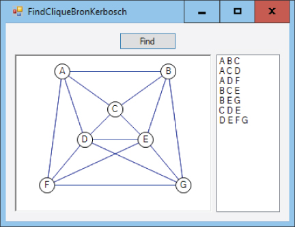
Figure 14.19: This program uses the Bron–Kerbosch algorithm to find maximal cliques.
- Build a program that checks local links to find a network's triangles.
- Recall the method for building communities by expanding maximal cliques. For example, suppose that you have found a maximal clique containing 15 softball players. You consider the neighbors of those nodes and add those that are adjacent to many of the clique's nodes. For example, if Amanda is a neighbor to 12 of the 15 softball player nodes, then she probably belongs in that community.
Now consider two adjacent communities. For example, suppose Amanda is also a member of a book club. Will growing the softball team and book club cliques make them merge into one community? Would that be good or bad?
- Suppose that you use clique percolation to build communities. You start with a k-clique and expand it M times where
 .
.
- How many nodes does that community contain?
- How far apart could two nodes be in the community?
- How close together could the farthest nodes be?
- If you expand the community k times, how far apart could two nodes be?
- If you expand the community k times, how close together could the farthest nodes be?
- Explain intuitively why a network cannot have an Eulerian cycle unless all of its nodes have even degree.
- Explain intuitively why a network cannot have an Eulerian path unless it has two or fewer nodes with odd degree.
- Can a network have exactly one node with an odd degree?
- Consider an M × N lattice of nodes where each node is connected by a link to its neighbors to the north, south, east, and west. What values for M and N will allow you to find an Eulerian cycle? What values will allow you to find an Eulerian path?
- Write a program that uses Hierholzer's algorithm to find an Eulerian cycle in a network.