CHAPTER 15
String Algorithms
String operations are common in many programs, so they have been studied extensively, and many programming libraries have good string tools. Because these operations are so important, the tools available to you probably use the best algorithms available, so you are unlikely to beat them with your own code.
For example, the Boyer–Moore algorithm described in this chapter lets you find the first occurrence of a string within another string. Because this is such a common operation, most high-level programming languages have tools for doing this. (In C#, that tool is the string class's IndexOf method. In Python, it's a string variable's find method.)
Those tools probably use some variation of the Boyer–Moore algorithm, so your implementation is unlikely to be much better. In fact, many libraries are written in assembly language or at some other very low level, so they may give better performance even if you use the same algorithm in your code.
If your programming library includes tools to perform these tasks, use them. The algorithms explained in this chapter are presented because they are interesting, form an important part of a solid algorithmic education, and provide examples of useful techniques that you may be able to adapt for other purposes.
Matching Parentheses
Some string values, such as arithmetic expressions, can contain nested parentheses. For proper nesting of parentheses, you can place a pair of matching parentheses inside another pair of matching parentheses, but you cannot place one parenthesis of a pair inside another matched pair. For example, ()(()(())) is properly nested, but (() and (())) are not.
Graphically, you can tell that an expression's parentheses are properly nested if you can draw lines connecting left and right parentheses so that every parenthesis is connected to another, all of the lines are on the same side (top or bottom) of the expression, and no lines intersect. Figure 15.1 shows that ()(()(())) is properly nested, but (() and (())) are not.

Figure 15.1: Lines connect matching pairs of parentheses.
Algorithmically, it is easy to see whether parentheses are properly matched by using a counter to keep track of the number of unmatched opening parentheses. Initialize the counter to 0, and loop through the expression. When you find an opening parenthesis, add 1 to the counter. When you find a closing parenthesis, subtract 1 from the counter. If the counter ever drops below 0, the parentheses are improperly nested. When you finish checking the expression, if the counter is not 0, the parentheses are improperly nested.
The following pseudocode shows the algorithm:
Boolean: IsProperlyNested(String: expression)Integer: counter = 0For Each ch In expressionIf (ch == '(') Then counter = counter + 1Else If (ch == ')') Thencounter = counter - 1If (counter < 0) Then Return FalseEnd IfNext chIf (counter == 0) Then Return TrueElse Return FalseIsProperlyNested
For example, when the algorithm scans the expression ()(()(())), the counter's values after reading each character are 1, 0, 1, 2, 1, 2, 3, 2, 1, 0. The counter never drops below 0, and it ends at 0, so the expression is nested properly.
Some expressions contain text other than parentheses. For example, the arithmetic expression ![]() contains numbers, operators such as × and +, and parentheses. To see whether the parentheses are nested properly, you can use the previous
contains numbers, operators such as × and +, and parentheses. To see whether the parentheses are nested properly, you can use the previous IsProperlyNested algorithm, ignoring any characters that are not parentheses.
Evaluating Arithmetic Expressions
You can recursively define a fully parenthesized arithmetic expression as one of the following:
- A literal value such as 4 or 1.75
- An expression surrounded by parentheses (expr) for some expression expr
- Two expressions separated by an operator, as in expr1 + expr2 or expr1 × expr2
For example, the expression ![]() uses the third rule, with the two expressions 8 and 3 separated by the operator ×. The values 8 and 3 are both expressions according to the first rule.
uses the third rule, with the two expressions 8 and 3 separated by the operator ×. The values 8 and 3 are both expressions according to the first rule.
You can use the recursive definition to create a recursive algorithm for evaluating arithmetic expressions. The following steps describe the algorithm at a high level:
- If the expression is a literal value, use your programming language's tools to parse it and return the result. (In C#, use
double.Parse. In Python, use thefloatfunction.) - If the expression is of the form (expr), then remove the outer parentheses, recursively use the algorithm to evaluate expr, and return the result.
- If the expression is of the form expr1?expr2 for expressions expr1 and expr2 and operator?, then recursively use the algorithm to evaluate expr1 and expr2, combine those values appropriately for the operator?, and return the result.
The basic approach is straightforward. Probably the hardest part is determining which of the three cases applies and breaking the expression into two operands and an operator in case 3. You can do that by using a counter similar to the one used by the IsProperlyNested algorithm described in the preceding section.
When the counter is 0, if you find an operator, case 3 applies and the operands are on either side of the operator.
If you finish scanning the expression and you don't find an operator when the counter is 0, then either case 1 or case 2 applies. If the first character is an opening parenthesis, then case 2 applies. If the first character is not an opening parenthesis, then case 1 applies.
Building Parse Trees
The algorithm described in the preceding section parses arithmetic expressions and then evaluates them, but you might like to do other things with an expression after you parse it. For example, suppose that you need to evaluate an expression that contains variables such as ![]() many times for different values of
many times for different values of ![]() , perhaps to draw a graph of the equation
, perhaps to draw a graph of the equation ![]() . One approach would be to use the previous algorithm repeatedly to parse and evaluate the expression, substituting different values for
. One approach would be to use the previous algorithm repeatedly to parse and evaluate the expression, substituting different values for ![]() . Unfortunately, parsing text is relatively slow.
. Unfortunately, parsing text is relatively slow.
Another approach is to parse the expression but not evaluate it right away. Then you can evaluate the preparsed expression many times with different values for ![]() without needing to parse the expression again. You can do this using an algorithm very similar to the one described in the preceding section. Instead of making the algorithm combine the results of recursive calls to itself, however, it builds a tree containing objects that represent the expression.
without needing to parse the expression again. You can do this using an algorithm very similar to the one described in the preceding section. Instead of making the algorithm combine the results of recursive calls to itself, however, it builds a tree containing objects that represent the expression.
For example, to represent multiplication, the algorithm makes a node with two children, where the children represent the multiplication's operands. Similarly, to represent addition, the algorithm makes a node with two children, where the children represent the addition's operands.
You can build a class for each of the necessary node types. The classes should provide an Evaluate method that calculates and returns the node's value, calling the Evaluate method for its child nodes if it has any.
Having built the parse tree, you can call the root node's Evaluate method any number of times for different values of ![]() .
.
Figure 15.2 shows the parse tree for the expression ![]() .
.

Figure 15.2: You can use parse trees to represent expressions such as  .
.
Pattern Matching
The algorithms described in the preceding sections are useful and effective, but they're tied to the particular application of parsing and evaluating arithmetic expressions. Parsing is a common task in computer programming, so it would be nice to have a more general approach that you could use to parse other kinds of text.
For example, a regular expression is a string that a program can use to represent a pattern for matching in another string. Programmers have defined several different regular expression languages. To keep this discussion reasonably simple, this section uses a language that defines the following symbols:
- An alphabetic character such as A or Q represents that letter.
- The
+symbol represents concatenation. For the sake of readability, this symbol is often omitted, so ABC is the same as . However, it may be convenient to require the symbol to make it easier for a program to parse the regular expression.
 - The
*symbol means that the previous expression can be repeated any number of times (including zero). - The
|symbol means that the text must match either the previous or the following expression. - Parentheses determine the order of operation.
For example, with this restricted language, the regular expression ![]() matches strings that begin with an A, contain any number of Bs, and then end with an A. That pattern would match ABA, ABBBBA, and AA.
matches strings that begin with an A, contain any number of Bs, and then end with an A. That pattern would match ABA, ABBBBA, and AA.
More generally, a program might want to find the first occurrence of a pattern within a string. For example, the string AABBA matches the previous pattern ![]() starting at the second letter.
starting at the second letter.
To understand the algorithms described here for regular expression matching, it helps to understand deterministic finite automata and nondeterministic finite automata. The following two sections describe deterministic and nondeterministic finite automata. The section after that explains how you can use them to perform pattern matching with regular expressions.
DFAs
A deterministic finite automaton (DFA), also known as a deterministic finite state machine, is basically a virtual computer that uses a set of states to keep track of what it is doing. At each step, it reads some input and, based on that input and its current state, moves into a new state. One state is the initial state in which the machine starts. One or more states can also be marked as accepting states.
If the machine ends its computation in an accepting state, then the machine accepts the input. In terms of regular expression processing, if the machine ends in an accepting state, the input text matches the regular expression.
In some models, it's convenient for the machine to accept its input if it ever enters an accepting state.
You can represent a DFA with a state transition diagram, which is basically a network in which circles represent states and directed links represent transitions to new states. Each link is labeled with the inputs that make the machine move into the new state. If the machine encounters an input that has no corresponding link, then it halts in a nonaccepting state.
To summarize, there are three ways that a DFA can stop:
- It can finish reading its inputs while in an accepting state. In that case, it accepts the input. (The regular expression matches.)
- It can finish reading its inputs while in a nonaccepting state. In that case, it rejects the input. (The regular expression does not match.)
- It can read an input that does not have a link leading out of the current state node. In that case, it rejects the input. (The regular expression does not match.)
For example, Figure 15.3 shows a state transition diagram for a DFA that recognizes the pattern ![]() . The DFA starts in state 0. If it reads an A character, then it moves to state 1. If it sees any other character, then the machine halts in a nonaccepting state.
. The DFA starts in state 0. If it reads an A character, then it moves to state 1. If it sees any other character, then the machine halts in a nonaccepting state.

Figure 15.3: This network represents the state transitions for a DFA that recognizes the pattern  .
.
Next, if the DFA is in state 1 and it reads a B, then it follows the loop and returns to state 1. If the DFA is in state 1 and reads an A, then it moves to state 2. If the DFA is in state 1 and reads any character other than A or B, then it halts in a nonaccepting state.
State 2 is marked with a double circle to indicate that it is an accepting state. Depending on how you are using the DFA, just entering this state might make the machine return a successful match. Alternatively, it might need to finish reading its input in that state, so if the input string contains more characters, the match fails.
For another example, consider the state transition diagram shown in Figure 15.4. This diagram represents a machine that matches a string that consists of AB repeated any number of times or BA repeated any number of times.

Figure 15.4: This network represents the state transitions for a DFA that recognizes the pattern  .
.
Programmatically, you can implement a DFA by making an object to represent each of the states in the state transition diagram. When presented with an input, the program moves from the current object to the object that is appropriate for that input.
Often, DFAs are implemented with a table showing the state transitions. For example, Table 15.1 shows the state transitions for the state transition diagram shown in Figure 15.3.
Table 15.1: A State Transition Table for ![]()
| STATE | 0 | 1 | 1 | 2 |
| On input | A | A | B | |
| New state | 1 | 2 | 1 | |
| Accepting? | No | No | No | Yes |
Building DFAs for Regular Expressions
You can translate simple regular expressions into transition diagrams and transition tables easily enough by using intuition, but for complicated regular expressions, it's nice to have a methodical approach. Then you can apply this approach to let a program do the work for you.
To convert a regular expression into a DFA state transition table, you can build a parse tree for the regular expression and then use it to generate recursively the corresponding state transitions.
The parse tree's leaves represent literal input characters such as A and B. The state transition diagram for reading a single input character is just a start state connected to an accepting final state with a link labeled by the required character. Figure 15.5 shows the simple state transition diagram for reading the input character B.

Figure 15.5: This transition diagram represents the simple regular expression B.
The parse tree's internal nodes represent the operators +, *, and |.
To implement the + operator, take the accepting state of the left subtree's transition diagram and make it coincide with the starting state of the right subtree's transition diagram, so the machine must perform the actions of the left subtree followed by the actions of the right subtree. For example, Figure 15.6 shows the transition diagrams for the simple literal patterns A and B on the left and the combined pattern ![]() on the right.
on the right.

Figure 15.6: The transition diagram on the right represents the regular expression  .
.
To implement the * operator, make the single subexpression's accepting state coincide with the subexpression's starting state. Figure 15.7 shows the transition diagram for the pattern ![]() on the left and the pattern
on the left and the pattern ![]() on the right.
on the right.

Figure 15.7: The transition diagram on the right represents the regular expression  .
.
Finally, to implement the | operator, make the starting and ending states of the left and right subexpressions' transition diagram coincide. Figure 15.8 shows the transition diagram for the patterns ![]() and
and ![]() on the left and the combined pattern
on the left and the combined pattern ![]() on the right.
on the right.
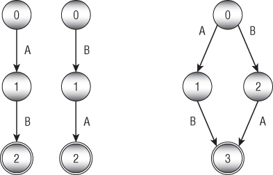
Figure 15.8: The transition diagram on the right represents the regular expression  .
.
This approach works in this instance, but it has a serious drawback under some conditions. What happens to the | operator if the two subexpressions start with the same input transitions? For example, suppose the two subexpressions are ![]() and
and ![]() . In that case, blindly following the previous discussion leads to the transition diagram on the left in Figure 15.9. It has two links labeled A that leave state 0. If the DFA is in state 0 and encounters input character A, which link should it follow?
. In that case, blindly following the previous discussion leads to the transition diagram on the left in Figure 15.9. It has two links labeled A that leave state 0. If the DFA is in state 0 and encounters input character A, which link should it follow?

Figure 15.9: These transition diagrams represent the regular expression  .
.
One solution is to restructure the diagram a bit, as shown on the right in Figure 15.9, so that the diagrams for the two subexpressions share their first state (state 1). This works, but it requires some cleverness—something that can be hard to build into a program. If the subexpressions were more complicated, finding a similar solution might be difficult—at least for a program.
One solution to this problem is to use an NFA instead of a DFA.
NFAs
A deterministic finite automaton is called deterministic because its behavior is completely determined by its current state and the input that it sees. If a DFA using the transition diagram on the right side of Figure 15.8 is in state 0 and reads the character B, it moves into state 2 without question.
A nondeterministic finite automaton (NFA) is similar to a DFA, except that multiple links may be leaving a state for the same input, as shown on the left in Figure 15.9. When that situation occurs during processing, the NFA is allowed to guess which path it should follow to eventually reach an accepting state. It's as if the NFA were being controlled by a fortune-teller who knows what inputs will come later and can decide which links to follow to reach an accepting state.
Of course, in practice a computer cannot really guess which state it should move into to eventually find an accepting state. What it can do is to try all of the possible paths. To do that, a program can keep a list of states it might be in. When it sees an input, the program updates each of those states, possibly creating a larger number of states.
Another way to think of this is to regard the NFA as simultaneously being in all of the states. If any of its current states is an accepting state, the NFA as a whole is in an accepting state.
You can make one more change to an NFA's transitions to make it slightly easier to implement. The operations shown in Figures 15.6 through 15.9 require that you make states from different subexpressions coincide—and that can be awkward.
An alternative is to introduce a new kind of null transition that occurs without any input. If the NFA encounters a null transition, it immediately follows it.
Figure 15.10 shows how you can combine state transition machines for subexpressions to produce more-complex expressions. Here the Ø character indicates a null transition, and a box indicates a possibly complicated network of states representing a subexpression.

Figure 15.10: Using an NFA and null transitions makes combining subexpressions more straightforward.
The first part of Figure 15.10 shows a set of states representing some subexpression. This could be as simple as a single transition that matches a single input, as shown in Figure 15.5, or it could be a complicated set of states and transitions. The only important feature of this construct from the point of view of the rest of the states is that it has a single input state and a single output state.
The second part of Figure 15.10 shows how you can combine two machines, ![]() and
and ![]() , by using the
, by using the + operator. The output state from ![]() is connected by a null transition to the input state of
is connected by a null transition to the input state of ![]() . By using a null transition, you avoid the need to make
. By using a null transition, you avoid the need to make ![]() 's output state and
's output state and ![]() 's input state coincide.
's input state coincide.
The third part of Figure 15.10 shows how you can add the * operator to ![]() .
. ![]() 's output state is connected to its input state by a null transition. The
's output state is connected to its input state by a null transition. The * operator allows whatever it follows to occur any number of times, including zero times, so another null transition allows the NFA to jump to the accept state without matching whatever is inside the M1.
The final part of Figure 15.10 shows how you can combine two machines ![]() and
and ![]() by using the
by using the | operator. The resulting machine uses a new input state connected by null transitions to the input states of ![]() and
and ![]() . The output states of
. The output states of ![]() and
and ![]() are connected by null transitions to a final output state for the new combined machine.
are connected by null transitions to a final output state for the new combined machine.
To summarize, you can follow these steps to make a regular expression parser:
- Build a parse tree for the regular expression.
- Use the parse tree to recursively build the states for an NFA representing the expression.
- Start the NFA in state 0 and use it to process the input string one character at a time.
String Searching
The previous sections explained how you can use DFAs and NFAs to search for patterns in a string. Those methods are quite flexible, but they're also relatively slow. To search for a complicated pattern, an NFA might need to track a large number of states as it examines each character in an input string one at a time.
If you want to search a piece of text for a target substring instead of a pattern, there are faster approaches. The most obvious strategy is to loop over all of the characters in the text and see whether the target is at each position. The following pseudocode shows this brute-force approach:
// Return the position of the target in the text.Integer: FindTarget(String: text, String: target)For i = 0 To <last index of string>// See if the target begins at position i.Boolean: found_it = TrueFor j = 0 To <last index of target>If (string[i + j] != target[j]) Then found_it = FalseNext j// See if we found the target.If (found_it) Then Return iNext i// If we got here, the target isn't present.Return -1End FindTarget
In this algorithm, variable i loops over the length of the text. For each value of i, the variable j loops over the length of the target. If the text has length ![]() and the target has length
and the target has length ![]() , the total run time is
, the total run time is ![]() . This is simpler than using an NFA, but it's still not very efficient.
. This is simpler than using an NFA, but it's still not very efficient.
The Boyer–Moore algorithm uses a different approach to search for target substrings much more quickly. Instead of looping through the target's characters from the beginning, it examines the target's characters starting at the end and works backward toward the beginning.
The easiest way to understand the algorithm is to imagine the target substring sitting below the text at a position where a match might occur. The algorithm compares characters starting at the target's leftmost character. If it finds a position where the target and text don't match, the algorithm slides the target to the right to the next position where a match might be possible.
For example, suppose you want to search the string A man a plan a canal Panama for the target string Roosevelt. Consider Figure 15.11.

Figure 15.11: Searching A man a plan a canal Panama for Roosevelt requires only three comparisons.
The algorithm first aligns the two strings so that they line up on the left and compares the last character in the target to the corresponding character in the text. At that position, the target's last character is t, and the text's corresponding character is p. Those characters don't match, so the algorithm slides the target to the right to find the next position where a match is possible. The text's character p doesn't appear anywhere in the target, so the algorithm slides the target to the right all the way past its current location, nine characters to the right.
At the new position, the target's last character is t, and the text's corresponding character is n. Again, the characters don't match, so the algorithm slides the target to the right. Again, the text's character n doesn't appear in the target, so the algorithm slides the target nine characters to the right.
At the new position, the target's last character is t, and the text's corresponding character is a. The characters don't match, so the algorithm slides the target to the right. Again, the text's character a doesn't appear in the target, so the algorithm slides the target nine characters to the right.
At this point, the target extends beyond the end of the text, so a match isn't possible, and the algorithm concludes that the target is not present in the text. The brute-force algorithm described earlier would have required 37 comparisons to decide that the target wasn't present, but the Boyer–Moore algorithm required only three comparisons.
Things don't always work out this smoothly. For a more complicated example, suppose that you want to search the text abba daba abadabracadabra for the target cadabra. Consider Figure 15.12.

Figure 15.12: Searching abba daba abadabracadabra for cadabra requires 18 comparisons.
The algorithm starts with the two strings aligned at the left and compares the target character a with the text character a. Those characters match, so the algorithm considers the preceding characters, r and d. Those characters do not match, so the algorithm slides the target to the right. In this case, however, the text's character d does appear in the target, so there's a chance that the d is part of a match. The algorithm slides the target to the right until the last d in the target (shown with a dark box in Figure 15.12) aligns with the d in the text.
At the new position, the target's last character is a, and the text's corresponding character is a space. Those characters don't match, so the algorithm slides the target to the right. The target has no space, so the algorithm moves the target its full width of seven characters.
At the new position, the target's last character is a and the text's corresponding character is r. Those characters don't match, so the algorithm slides the target to the right. The character r does appear in the target, so the algorithm moves the target until its last r (dark) aligns with the r in the text.
At the new position, the target's last character is a, and the text's corresponding character is a. These characters match, so the algorithm compares the preceding characters to see whether they match. Those characters also match, so the algorithm continues comparing characters backward through the target and text. Six characters match. Not until the algorithm considers the target's first character does it find a mismatch. Here the target's character is c, and the text's corresponding character is b.
The target has a b, but it comes after the position in the target the algorithm is currently considering. To align this b with the one in the text, the algorithm would have to move the target to the left. All leftward positions have already been eliminated as possible locations for the match, so the algorithm doesn't do this. Instead, it shifts the target seven characters to the right to the next position where a match could occur.
At this new position, the target's characters all match the corresponding characters in the text, so the algorithm has found a match.
The following steps describe the basic Boyer–Moore algorithm at a high level:
- Align the target and text on the left.
- Repeat until the target's last character is aligned beyond the end of the text:
- Compare the characters in the target with the corresponding characters in the text, starting from the end of the target and moving backward toward the beginning.
- If all of the characters match, then congratulations—you've found a match!
- Suppose character
Xin the text doesn't match the corresponding character in the target. Slide the target to the right until theXaligns with the next character with the same valueXin the target to the left of the current position. If no such characterXexists to the left of the position in the target, slide the target to the right by its full length.
One of the more time-consuming pieces of this algorithm is step 2c, which calculates the amount by which the algorithm slides the target to the right. You can make this step faster if you precalculate the amounts for different mismatched characters in different positions within the target.
For example, suppose that the algorithm compares target and text characters, and the first mismatch is in position 3, where the text has the character G. The algorithm would then slide the text to the right to align the G with the first G that appears to the left of position 3 in the target. If you use a table to store the amounts by which you need to slide the target, then you can just look up that amount instead of calculating it during the search.
The Boyer–Moore algorithm has the unusual property that it tends to be faster if the target string is longer because, when it finds a nonmatching character, it can shift the target farther.
Calculating Edit Distance
The edit distance of two strings is the minimum number of changes that you need to make to turn the first string into the second. You can define the changes that you are allowed to make in several ways. For this discussion, assume that you are only allowed to remove or insert letters. (Another common change that isn't considered here is changing one letter into another letter. You can achieve the same result by deleting the first character and then inserting the second.)
For example, consider the words encourage and entourage. It's fairly easy to see that you can change encourage into entourage by removing the c and inserting a t. That's two changes, so the edit distance between those two words is 2.
For another example, consider the words assent and descent. One way to convert assent into descent would be to follow these steps:
- Remove a to get ssent.
- Remove s to get sent.
- Remove s to get ent.
- Add d to get dent.
- Add e to get deent.
- Add s to get desent.
- Add c to get descent.
This requires seven steps, so the edit distance is no more than 7, but how can you tell if this is the most efficient way to convert assent to descent? For longer words or strings (or, as you'll see later in this section, for files), it can be hard to be sure that you have found the best solution.
One way to calculate the edit distance is to build an edit graph that represents all the possible changes that you could make to get from the first word to the second. Start by creating an array of nodes similar to the one shown in Figure 15.13.

Figure 15.13: This edit graph represents possible ways to convert assent to descent.
The nodes across the top of the graph represent the letters in the first word. The nodes down the left side represent the letters in the second word. Create links between the nodes leading to their rightward and downward neighbors.
Add diagonal links ending at any locations where the corresponding letters in both words are the same. For example, assent has an e in the fourth position, and descent has an e in its second position, so a diagonal link leads to the node below the e in assent and to the right of the first e in descent.
Each link represents a transformation of the first word, making it more similar to the second word. A link pointing right represents removing a letter from the first word. For example, the link leading to the a on the top row represents removing the a from assent, which would make ssent.
A link pointing down represents adding a letter to the word. For example, the link pointing to the d in the first column represents adding the letter d to the current word, which would make dassent.
A diagonal link represents keeping a letter unchanged.
Any path through the graph from the upper-left corner to the lower-right corner corresponds to a series of changes to convert the first word into the second. For example, the bold arrows shown in Figure 15.13 represent the changes described earlier to convert assent into descent.
Now finding a path through the edit graph that has the least cost is fairly easy. Give each horizontal and vertical link a cost of 1, and give the diagonal links a cost of 0. Now you just need to find the shortest path through the network.
You can use the same techniques described in Chapter 13, “Basic Network Algorithms,” to find the shortest path, but this network has a special structure that lets you use an easier method.
First, set the distances for the nodes in the top row to be their column numbers. To get to the node in column 5 from the upper-left corner, you need to cross five links, so its distance is 5.
Similarly, set the distances for the nodes in the leftmost column to be their row numbers. To get to the node in row 7, you need to cross seven links, so its distance is 7.
Now loop over the rows and, for each row, loop over its columns. The shortest path to the node at position ![]() comes via the node above at
comes via the node above at ![]() , the node to the left at
, the node to the left at ![]() , or, if a diagonal move is allowed, the node diagonally up and to the left at
, or, if a diagonal move is allowed, the node diagonally up and to the left at ![]() . The distances to all of those nodes have already been set. You can determine what the cost would be for each of those possibilities and set the distance for the node at
. The distances to all of those nodes have already been set. You can determine what the cost would be for each of those possibilities and set the distance for the node at ![]() to be the smallest of those.
to be the smallest of those.
When you're finished looping through the rows and columns, the distance to the node in the lower-right corner gives the edit distance.
Once you know how to find the edit distance between two words or strings, it's easy to find the edit distance between two files. You could just use the algorithm as is to compare the files character by character. Unfortunately, that could require a very large edit graph. For example, if the two files have about 40,000 characters (this chapter is in that neighborhood), then the edit graph would have about ![]() . Building that graph would require a lot of memory, and using it would take a long time.
. Building that graph would require a lot of memory, and using it would take a long time.
Another approach is to modify the algorithm so that it compares lines in the files instead of characters. If the files each contain about ![]() , the edit graph would hold about
, the edit graph would hold about ![]() . That's still a lot, but it's much more reasonable.
. That's still a lot, but it's much more reasonable.
Phonetic Algorithms
A phonetic algorithm is one that categorizes and manipulates words based on their pronunciation. For example, suppose you are a customer service representative and a customer tells you that his name is Smith. You need to look up that customer in your database, but you don't know if the name should be spelled, Smith, Smyth, Smithe, or Smythe.
If you enter any reasonable spelling (perhaps Smith), the computer can convert it into a phonetic form and then look for previously stored phonetic versions in the customer database. You can look through the results, ask a few questions to verify that you have the right person, and begin troubleshooting.
Unfortunately, deducing a word's pronunciation from its spelling it difficult, at least in English. That means these algorithms tend to be long and complicated.
The following sections describe two phonetic algorithms: Soundex and Metaphone.
Soundex
The Soundex algorithm was devised by Robert C. Russell and Margaret King Odell in the early 1900s to simplify the U.S. census. They first patented their algorithm in 1918, long before the first computers were created.
The following list shows my version of the Soundex rules. They're slightly different from the rules that you'll see online. I've reformulated them slightly to make them easier to implement.
- Save the first letter of the name for later use.
- Remove w and h after the first character.
- Use Table 15.2 to convert the remaining characters into codes. If a character doesn't appear in the table (w or h), leave it unchanged.
Table 15.2: Soundex Letter Codes
LETTER CODE a, e, I, o, u, y 0 b, f, p, v 1 c, g, j, k, q, s, x, z 2 d, t 3 l 4 m, n 5 r 6 - If two or more adjacent codes are the same, keep only one of them.
- Replace the first code with the original first letter.
- Remove code 0 (vowels after the first letter).
- Truncate or pad with 0s on the right so that the result has four characters.
For example, let's walk through the steps for the name Ashcraft.
- We save the first letter, A.
- We remove w and h after the first letter to get Ascraft.
- Using Table 15.2 to convert the remaining letters into codes gives 0226013.
- Removing adjacent duplicates gives 026013.
- Replacing the first code with the original first letter gives A26013.
- Removing code 0 gives A2613.
- Truncating to four characters gives the final code A261.
Over the years, there have been several variations on the original Soundex algorithm. Most SQL database systems use a slight variation that does not consider vowels when looking for adjacent codes. For example, in the name Alol, the two Ls are separated by a vowel. Basic Soundex would convert them into the code, 4, and keep them both. SQL Soundex would remove the vowel, find the two adjacent 4s, and remove one of them.
Another relatively simple variation of the original algorithm uses the character codes shown in Table 15.3.
Table 15.3: Refined Soundex Letter Codes
| LETTER | CODE |
| b, p | 1 |
| f, v | 2 |
| c, k, s | 3 |
| g, j | 4 |
| q, x, z | 5 |
| d, t | 6 |
| l | 7 |
| m, n | 8 |
| r | 9 |
Still other examples include variations designed for use with non-English names and words. The Daitch–Mokotoff Soundex (D-M Soundex) was designed to represent Germanic and Slavic names better. Those kinds of variations tend to be much more complicated than the original Soundex algorithm.
Metaphone
In 1990, Lawrence Philips published a new phonetic algorithm named Metaphone. It uses a more complex set of rules to represent English pronunciation more accurately. The following list shows the Metaphone rules:
- Drop duplicate adjacent letters, except for C.
- If the word starts with KN, GN, PN, AE, WR, drop the first letter.
- If the words ends with MB, drop the B.
- Convert C:
- Convert C into K if part of SCH.
- Convert C into X if followed by IA or H.
- Convert C into S if followed by I, E, or Y.
- Convert all other Cs into K.
- Convert D:
- Convert C into J if followed by GE, GY, or GI.
- Convert C into T otherwise.
- Convert G:
- Drop the G if part of GH unless it is at the end of the word or it comes before a vowel.
- Drop the G in GN and GNED at the end of the word.
- Convert G into J if part of GI, GE, or GY and not in GG.
- Convert all other Gs into K.
- If H comes after a vowel and not before a vowel, drop it.
- Convert CK into K.
- Convert PH into F.
- Convert Q into K.
- Convert S into X if followed by H, IO, or IA.
- Convert T:
- Convert T into X if part of TIA or TIO.
- Convert TH into 0.
- Drop the T in TCH.
- Convert V into F.
- Convert WH into W if at the beginning of the word. Otherwise, drop the Ws if not followed by a vowel.
- Convert X:
- Convert X into S if at the beginning of the word.
- Otherwise convert X into KS.
- Drop Y if not followed by a vowel.
- Convert Z into S.
- Drop all remaining vowels after the first character.
Metaphone is an improvement over Soundex, but it also has several variations. For example, Double Metaphone is the second version of the original Metaphone algorithm. It is called Double Metaphone because it can generate primary and secondary codes for words to differentiate between words that have the same primary code.
Metaphone 3 further refines Metaphone's phonetic rules and provides better results with non-English words that are common in the United States and some common names. It is available as a commercial product. There are also versions that handle Spanish and German pronunciations.
For more information on phonetic algorithms, see the following URLs:
Summary
Many programs need to examine and manipulate strings. Even though programming libraries include many string manipulation tools, it's worth knowing how some of those algorithms work. For example, using a regular expression tool is much easier than writing your own, but the technique of using DFAs and NFAs to process commands is useful in many other situations. The Boyer–Moore string search algorithm is a well-known algorithm that any student of algorithms should see at least once. Edit distance algorithms let you determine how close two words, strings, or even files are to each other and to find the differences between them. Finally, Soundex and other phonetic algorithms are useful for finding names or other words when you're unsure of their spelling.
One kind of string algorithm that isn't covered in this chapter is algorithms used for encryption and decryption. The next chapter describes some of the more important and interesting algorithms used to encrypt and decrypt strings and other data.
Exercises
You can find the answers to these exercises in Appendix B. Asterisks indicate particularly difficult problems. Problems with two asterisks are exceptionally hard or time-consuming.
- Write a program that determines whether an expression entered by the user contains properly nested parentheses. Allow the expression to contain other characters as well, as in
 .
. - Write a program that parses and evaluates arithmetic expressions that contain real numbers and the operators
+,–,*, and/. - How would you modify the program you wrote for the preceding exercise to handle the unary negation operator, as in
 ?
? - How would you modify the program you wrote for Exercise 2 to handle functions such as sine, as in
 ?
? - Write a program that parses and evaluates Boolean expressions such as
 , where
  means True,
  means False, & means AND, | means OR, and – means NOT.
 - **Write a program similar to the one shown in Figure 15.14. The program should build a parse tree for the expression entered by the user and then graph it. (Depending on how your program draws the graphics, the default coordinate system for the picture probably will have (0, 0) in the upper-left corner, and coordinates will increase to the right and down. The coordinate system may also use one unit in the X and Y directions per pixel, which means that the resulting graph will be fairly small. Unless you have experience with graphics programming, don't worry about scaling and transforming the result to fit the form nicely.)

Figure 15.14: This program, GraphExpression, builds a parse tree for an expression and then evaluates it many times to graph the expression. - Build a state transition table for the DFA state transition diagram shown in Figure 15.4.
- Draw a state transition diagram for a DFA to match the regular expression ((AB)|(BA))*.
- Build a state transition table for the state transition diagram you drew for the preceding exercise.
- *Write a program that lets the user type a DFA's state transitions and an input string and determines whether the DFA accepts the input string.
- Do you think it would be better for a DFA to get its state transitions from a table similar to the one shown in Table 15.1 or to use objects to represent the states? Why?
- How can you make a set of states for an NFA to see whether a pattern occurs anywhere within a string? For example, how could you determine whether the pattern ABA occurred anywhere within a long string? Draw the state transition diagram using a block to represent the pattern's machine (as done in Figure 15.10).
- Draw the parse tree for the expression
 . Then draw the NFA network you get by applying the rules described in this chapter to the parse tree.
 - Convert the NFA state transition diagram you drew for the preceding exercise into a simple DFA state transition diagram.
- Suppose that you want to search some text of length
 for a target substring of length
  . Find an example where a brute-force search requires
  steps.
 - Study the edit graph shown in Figure 15.13. What rule should you follow to find the least-cost path from the upper-left corner to the lower-right corner? What is the true edit distance?
- *Write a program that calculates edit distance.
- *Enhance the program you wrote for the preceding exercise to display the edits required to change one string into another. Display deleted characters as crossed out and inserted characters as underlined, as shown in Figure 15.15.

Figure 15.15: By following the path through the edit graph, you can show exactly what edits were needed to change one string into another. - Is edit distance commutative? In other words, is the edit distance between word 1 and word 2 the same as the edit distance between word 2 and word 1? Why or why not?
- *Modify the program you wrote for Exercise 17 to calculate the edit distance between two files instead of the differences between two strings.
- *Modify the program you wrote for Exercise 18 to display the differences between two files instead of the differences between two strings.
- Write a program that calculates Soundex encodings. When the program starts, make it verify that the names Smith, Smyth, Smithe, and Smythe all encode to S530. Also make the program verify the encoded values shown in Table 15.4.
Table 15.4: Soundex Encodings for Example Names
| NAME | SOUNDEX ENCODING |
| Robert | R163 |
| Rupert | R163 |
| Rubin | R150 |
| Ashcraft | A261 |
| Ashcroft | A261 |
| Tymczak | T522 |
| Pfister | P236 |
| Honeyman | H555 |