CHAPTER 10
Trees
This chapter explains trees, which are highly recursive data structures that you can use to store hierarchical data and model decision processes. For example, a tree can store a company organizational chart or the parts that make up a complex machine such as a car.
This chapter explains how to build relatively simple trees and provides the background that you need to understand the more complicated trees described in Chapter 11 and Chapter 12.
Tree Terminology
Tree terminology includes a hodgepodge of terms taken from genealogy, horticulture, and computer science. Trees use a lot of terms, but many of them are intuitive because you probably already understand what they mean in another context.
A tree consists of nodes connected by branches. Usually, the nodes contain some sort of data, and the branches do not.
The branches in a tree are usually directed so that they define a parent-child relationship between the nodes that they connect. Normally, branches are drawn as arrows pointing from the parent node to the child node. Two nodes that have the same parent are sometimes called siblings.
Each node in the tree has exactly one parent node, except for a single, unique root node, which has no parent.
The children, the children's children, and so on, for a node are that node's descendants. A node's parent, its parent's parent, and so on, up to the root are that node's ancestors.
All of these relationship-oriented terms make sense if you think of the tree as a family tree. You can even define terms such as cousin, nephew, and grandparent without confusing anyone, although those terms are uncommon.
Depending on the type of tree, nodes may have any number of children. The number of children a node has is the node's degree. A tree's degree is the maximum degree of its nodes. For example, in a degree 2 tree, which is usually called a binary tree, each node can have at most two children.
A node with no children is called a leaf node or an external node. A node that has at least one child is called an internal node.
Unlike real trees, tree data structures usually are drawn with the root at the top and the branches growing downward, as shown in Figure 10.1.

Figure 10.1: Tree data structures usually are drawn with the root at the top.
All of these definitions explain what a tree is intuitively. You can also recursively define a tree to be either
- A single root node
- A root node connected by branches to one or more smaller trees
A node's level or depth in the tree is the distance from the node to the root. To think of this in another way, a node's depth is the number of links between it and the root node. In particular, the root's level is 0.
A node's height is the length of the longest path from the node downward through the tree to a leaf node. In other words, it's the distance from the node to the bottom of the tree.
A tree's height is the same as the height of the root node.
A subtree of a tree T rooted at the node R is the node R and all of its descendants. For example, in Figure 10.1, the subtree rooted at node 5 is the tree containing the nodes 5, 7, 6, and 8.
An ordered tree is one in which the order of the children is important in some way. For example, many algorithms treat the left and right children in a binary tree differently. An unordered tree is one in which the order of the children doesn't matter. (Usually, a tree has an ordering, even if it's not particularly important to the algorithm. This is true simply because the children or branches are stored in a list, array, or some other collection that imposes an ordering on them.)
For any two nodes, the lowest common ancestor (or first common ancestor) is the node that is the ancestor of both nodes that is closest to those nodes. Another way to think about this is to start at one node and move up toward the root until you reach the first node that is an ancestor of the other node. For example, in Figure 10.1, the lowest common ancestor of nodes 3 and 5 is the root 4.
Note that the lowest common ancestor of two nodes might be one of those two nodes. For example, in Figure 10.1, the lowest common ancestor of nodes 5 and 6 is node 5.
Note also that there is a unique path between any two nodes in a tree that doesn't cross any branch more than once. The path starts at the first node, moves up the tree to the nodes’ lowest common ancestor, and then moves down the tree to the second node.
A full tree is one in which every node has either zero children or as many children as the tree's degree. For example, in a full binary, every node has either zero or two children. The tree shown in Figure 10.1 is not full because node 5 has only one child.
A complete tree is one in which every level is completely full, except possibly the bottom level where all the nodes are pushed as far to the left as possible. Figure 10.2 shows a complete binary tree. Notice that this tree is not full because node I has only one child.

Figure 10.2: In a complete binary tree, every level is completely full, except possibly the bottom level, where the nodes are pushed as far to the left as possible.
A perfect tree is full, and all the leaves are at the same level. In other words, the tree holds every possible node for a tree of its height.
Figure 10.3 shows examples of full, complete, and perfect binary trees.

Figure 10.3: Full, complete, and perfect binary trees contain an increasing number of nodes for a given height.
That's a lot of terminology all at once, so Table 10.1 summarizes these tree terms to make remembering them a bit easier.
Table 10.1: Summary of Tree Terminology
| TERM | MEANING |
| Ancestor | A node's parent, grandparent, great grandparent, and so on, up to the root are the node's ancestors. |
| Binary tree | A tree with degree 2. |
| Branch | Connects nodes in a tree. |
| Child | A child node is connected to its parent in the tree. Normally, a child is drawn below its parent. |
| Complete tree | A tree in which every level is completely full, except possibly the bottom level, where all the nodes are pushed as far to the left as possible. |
| Degree | For a node, the number of children the node has. For a tree, the maximum degree of any of its nodes. |
| Depth | Level. |
| Descendant | A node's children, grandchildren, great grandchildren, and so on, are the node's descendants. |
| External node | A leaf node. |
| Lowest (or first) common ancestor | For any two nodes, the node that is the ancestor of both nodes that is closest to those nodes. |
| Full tree | A tree in which every node has either zero children or as many children as the tree's degree. |
| Height | For a node, the length of the longest path from the node downward through the tree to a leaf node. For a tree, this is the same as the root's height. |
| Internal node | A tree node that has at least one child. |
| Leaf node | A tree node with no children. |
| Level | A tree node's level is the distance (in links) between it and the root node. |
| Node | An object that holds data in a tree. Connected to other nodes by branches. |
| Ordered tree | A tree in which the ordering of each node's children matters. |
| Parent | A parent node is connected to its child nodes by branches. Every node has exactly one parent, except the root node, which has no parent. Normally, the parent is drawn above its children. |
| Perfect tree | A full tree where all of the leaves are at the same level. |
| Root | The unique node at the top of the tree that has no parent. |
| Sibling | Two nodes in a tree that have the same parent are siblings. |
| Subtree | A node and all of its descendants in a tree. |
Having learned all of these terms, you're ready to start learning some of the properties and uses of trees.
Binary Tree Properties
Binary trees are useful in many algorithms, partly because lots of problems can be modeled using binary choices and partly because binary trees are relatively easy to understand. The following are some useful facts about binary trees:
- The number of branches B in a binary tree containing N nodes is
 .
. - The number of nodes N in a perfect binary tree of height H is
 .
. - Conversely, if a perfect binary tree contains N nodes, it has a height of
 .
. - The number of leaf nodes L in a perfect binary tree of height H is
 . Because the total number of nodes in a perfect binary tree of height H is
  , the number of internal nodes I is
  .
. - This means that in a perfect binary tree, almost exactly half of the nodes are leaves, and almost exactly half are internal nodes. More precisely,
 .
. - The number of missing branches (places where a child could be added) M in a binary tree that contains N nodes is
 .
. - If a binary tree has
 leaf nodes and
  nodes with degree 2, then
  . In other words, there is one more leaf node than nodes with degree 2.
These facts often make it easier to calculate the run time for algorithms that work with trees. For example, if an algorithm must search a perfect binary tree containing N nodes from the root to a leaf node, then you know that the algorithm needs only ![]() steps.
steps.
If a binary tree containing N nodes is fat (isn't too tall and skinny), such as if it's a complete tree, its statistics are similar to those of a perfect binary tree in terms of Big O notation. For example, if a fat binary tree contains N nodes, it has ![]() height,
height, ![]() leaves,
leaves, ![]() internal nodes, and O(N) missing branches.
internal nodes, and O(N) missing branches.
These properties are also true for fat trees of higher degrees but with different log bases. For example, a fat degree 10 tree containing N nodes has height ![]() . Because all log bases are the same in Big O notation, this is the same as
. Because all log bases are the same in Big O notation, this is the same as ![]() , although in practice the constants ignored by Big O notation may make a big difference.
, although in practice the constants ignored by Big O notation may make a big difference.
Chapter 11 describes balanced trees that do not to grow too tall and thin in order to guarantee that these properties are true.
Tree Representations
You can use a class to represent a tree's nodes. For complete trees, you can also store the tree in an array. The following two sections describe these approaches.
Building Trees in General
You can use a class to represent a tree's nodes much as you can use them to make the cells in a linked list. Give the class whatever properties it needs to hold data. Also give it object references to represent the branches to the node's children.
In a binary tree, you can use separate properties named LeftChild and RightChild for the branches.
The following pseudocode shows how you might create a binary node class. The details will differ depending on your programming language.
Class BinaryNodeString: NameBinaryNode: LeftChildBinaryNode: RightChildConstructor(String: name)Name = nameEnd ConstructorEnd Class
The class begins by declaring a public property called Name to hold the node's name. It then defines two properties named LeftChild and RightChild to hold references to the node's children.
The class's constructor takes a string as a parameter and saves it in the node's Name property.
The following pseudocode shows how you could use this class to build the tree shown in Figure 10.1:
BinaryNode: root = New BinaryNode("4")BinaryNode: node1 = New BinaryNode("1")BinaryNode: node2 = New BinaryNode("2")BinaryNode: node3 = New BinaryNode("3")BinaryNode: node5 = New BinaryNode("5")BinaryNode: node6 = New BinaryNode("6")BinaryNode: node7 = New BinaryNode("7")BinaryNode: node8 = New BinaryNode("8")root.LeftChild = node2root.RightChild = node5node2.LeftChild = node1node2.RightChild = node3node5.RightChild = node7node7.LeftChild = node6node7.RightChild = node8
This code first creates a BinaryNode object to represent the root. It then creates other BinaryNode objects to represent the tree's other nodes. After it has created all the nodes, the code sets the nodes’ left and right child references.
Sometimes, it may be useful to make the constructor take as parameters references to the node's children. If one of those values should be undefined, you can pass the value null, None, or your programming language's equivalent into the constructor. The following pseudocode shows how you might build the same tree if the constructor takes a node's children as parameters:
BinaryNode: node1 = New BinaryNode("1", null, null)BinaryNode: node3 = New BinaryNode("3", null, null)BinaryNode: node1 = New BinaryNode("6", null, null)BinaryNode: node3 = New BinaryNode("8", null, null)BinaryNode: node2 = New BinaryNode("2", node1, node3)BinaryNode: node7 = New BinaryNode("7", node6, node8)BinaryNode: node5 = New BinaryNode("5", null, node7)BinaryNode: root = New BinaryNode("4", node2, node5)
If the tree's degree is greater than 2 or if it is unordered (so that the order of a node's children is unimportant), it is usually more convenient to put the child references in an array, list, or some other collection. That lets the program loop through the children, doing something to each, instead of requiring you to write a separate line of code for each child.
The following pseudocode shows how you could create a TreeNode class that allows each node to have any number of children:
Class TreeNodeString: NameList Of TreeNode: ChildrenConstructor(String: name)Name = nameEnd ConstructorEnd Class
This class is similar to the preceding one, except that it stores its children in a List of references to TreeNode objects instead of in separate properties.
The following pseudocode shows another approach for creating a TreeNode class that allows nodes to have any number of children:
Class TreeNodeString: NameTreeNode: FirstChild, NextSiblingConstructor(String: name)Name = nameEnd ConstructorEnd Class
In this version, the FirstChild field provides a link to the first of the node's children. The NextSibling field is a link to the next sibling in the child nodes of this node's parent. Basically, this treats a node's child list as a linked list of nodes.
Figure 10.4 shows these two representations of trees where nodes can have any number of children. The version on the left is often easier to understand. However, the version on the right lets you treat child nodes as linked lists, so it may make rearranging children easier.

Figure 10.4: These are two representations of the same tree.
Occasionally, it may be useful to make a node class's constructor take a parameter giving the node's parent. It can then add the child to the parent's Children list.
Notice that these representations only have links from a node to its child nodes. They don't include a link from a node up to its parent. Most tree algorithms work in a top-down manner, so they move from parent to child down into the tree. If you really need to be able to find a node's parent, however, you can add a Parent property to the node class.
Most tree algorithms store data in each node, but a few store information in the branches. If you need to store information in the branches, you can add the information to the child nodes. The following pseudocode demonstrates this approach:
Class TreeNodeString: NameList Of TreeNode: ChildrenList Of Data: BranchDataConstructor(String: name)Name = nameEnd ConstructorEnd Class
Now when you add a node to the tree, you also need to add data for the branch that leads to that child.
Often, an algorithm will need to use the branch data to decide which path to take down through the tree. In that case, it can loop through a node's children and examine their branch data to pick the appropriate path.
Building Complete Trees
The heapsort algorithm described in Chapter 6 uses a complete binary tree stored in an array to represent a heap, a binary tree in which every node holds a value that is at least as large as the values in all of its children. Figure 10.5 shows a heap represented as a tree and stored in an array.

Figure 10.5: You can store a heap, or any complete binary tree, conveniently in an array.
If a node is stored at index i in the array, the indices of its children are ![]() and
and ![]() .
.
Conversely, if a node has index j, its parent has index ⌊![]() ⌋ where ⌊ ⌋
⌋ where ⌊ ⌋![]() means to truncate the result to the next-smaller integer. For example, ⌊
means to truncate the result to the next-smaller integer. For example, ⌊![]() ⌋ is 2 and ⌊
⌋ is 2 and ⌊![]() ⌋ is also 2.
⌋ is also 2.
This provides a concise format for storing any complete binary tree in an array. Working with this kind of tree can be a bit awkward and confusing, however, particularly if you need to resize the array frequently. For those reasons, you may want to stick to using classes to build trees.
Tree Traversal
One of the most basic and important tree operations is traversal. In a traversal, the goal is for the algorithm to visit all the nodes in the tree in some order and perform an operation on them. The most basic traversal simply enumerates the nodes so that you can see their ordering in the traversal.
Binary trees have four kinds of traversals.
- Preorder: This traversal visits a node before visiting its children.
- Inorder: This traversal visits a node's left child, then the node, then its right child.
- Postorder: This traversal visits a node's children before visiting the node.
- Breadth-first: This traversal visits all the nodes at a given level in the tree before visiting any nodes at lower levels.
Preorder, postorder, and breadth-first traversals make sense for any kind of tree. Inorder traversals are usually only defined for binary trees.
Because the preorder, inorder, and postorder traversals all dive deeply into the tree before backtracking up to visit other parts of the tree, they are sometimes called depth-first traversals.
The following sections describe the four kinds of traversals in greater detail.
Preorder Traversal
In a preorder traversal, the algorithm processes a node followed by its left child and then its right child. For example, consider the tree shown in Figure 10.6 and suppose that you're writing an algorithm simply to display the tree's nodes in a preorder traversal.

Figure 10.6: Traversals process a tree's nodes in different orders.
To produce the tree's preorder traversal, the algorithm first visits the root node, so it immediately outputs the value D. The algorithm then moves to the root node's left child.
It visits that node, so it outputs B and then moves to that node's left child.
There the algorithm outputs A. That node has no children, so the algorithm returns to the previous node, B, and visits that node's right child.
There the algorithm outputs C. That node also has no children, so the algorithm returns to the previous node, B. It has finished visiting that node's children, so the algorithm moves up the tree again to node D and visits that node's right child.
The algorithm outputs the next node, E. That node also has no children, so the algorithm returns to the previous node, which is the root node. It has finished visiting the root's children, so the algorithm is done producing the traversal.
The full traversal order is D, B, A, C, E.
Notice that the algorithm examines or visits the nodes in one order but processes the nodes to produce an output in a different order. The following list shows the series of steps the algorithm follows while producing the preorder traversal for the tree shown in Figure 10.6:
- Visit D
- Output D
- Visit B
- Output B
- Visit A
- Output A
- Visit B
- Visit C
- Output C
- Visit B
- Visit D
- Visit E
- Output E
- Visit D
The following pseudocode shows a natural recursive implementation of this algorithm:
TraversePreorder(BinaryNode: node)<Process node>If (node.LeftChild != null) Then TraversePreorder(node.LeftChild)If (node.RightChild != null) Then TraversePreorder(node.RightChild)End TraversePreorder
This algorithm simply follows the definition of a preorder traversal. It starts by processing the current node. In a real program, you would insert whatever code you needed to execute for each node here. For example, you might use code that adds the current node's label to an output string, you might examine the node to see whether you had found a particular target item, or you might add the node itself to an output list.
Next the algorithm determines whether the node has a left child. If it does, the algorithm calls itself recursively to traverse the left child's subtree. The algorithm then repeats that step for the right child and is done.
The algorithm is extremely short and simple.
To traverse the entire tree, a program would simply call TraversePreorder, passing it the root node as a parameter.
This algorithm works quite well, but its code must be placed somewhere in the program—perhaps in the main program, in a code module, or in a helper class. Usually, it is more convenient to place code that manipulates a tree inside its node class. The following pseudocode shows the same algorithm implemented inside the BinaryNode class:
Class BinaryNode…TraversePreorder()<Process this node>If (LeftChild != null) Then TraversePreorder(LeftChild)If (RightChild != null) Then TraversePreorder(RightChild)End TraversePreorderEnd Class
This is almost the same as the previous version, except that the code is running within a BinaryNode object, so it has direct access to that object's LeftChild and RightChild properties. This makes the code slightly simpler and keeps it nicely encapsulated within the BinaryNode class (thus making it more object-oriented'ish).
Now, to traverse the entire tree, you simply invoke the root node's TraversePreorder method.
Although this discussion is about binary trees, you can also define a preorder traversal for trees of higher degrees. The only rule is that you visit the node first and then visit its children.
Inorder Traversal
In an inorder traversal or symmetric traversal, the algorithm processes a node's left child, the node, and then the node's right child. For the tree shown in Figure 10.6, the algorithm starts at the root node and moves to its left child B. To process node B, the algorithm first moves to that node's left child A.
Node A has no left child, so the algorithm visits the node and outputs A. Node A also has no right child, so the algorithm returns to the parent node B.
Having finished with node B's left child, the algorithm processes node B and outputs B. It then moves to that node's right child C.
Node C has no left child, so the algorithm visits the node and outputs C. The node also has no right child, so the algorithm returns to the parent node B.
The algorithm has finished with node B's right child, so it returns to the root node D. The algorithm has finished with D's left child, so it outputs D and then moves to its right child E.
Node E has no left child, so the algorithm visits the node and outputs E. The node also has no right child, so the algorithm returns to the parent node D.
The full traversal order is A, B, C, D, E. Notice that this outputs the tree's nodes in sorted order. Normally the term sorted tree means that the tree's nodes are arranged so that an inorder traversal processes them in sorted order like this.
The following pseudocode shows a recursive implementation of this algorithm inside the BinaryNode class:
Class BinaryNode…TraverseInorder()If (LeftChild != null) Then TraverseInorder(LeftChild)<Process this node>If (RightChild != null) Then TraverseInorder(RightChild)End TraverseInorderEnd Class
This algorithm simply follows the definition of an inorder traversal. It recursively processes the node's left child if it exists, processes the node itself, and then recursively processes the node's right child if it exists.
To traverse the entire tree, a program would simply call the root node's TraverseInorder method.
Unlike the preorder traversal, it's unclear how you would define an inorder traversal for a tree with a degree greater than 2. You could define it to mean that the algorithm processes the first half of a node's children, then the node, and then the remaining children. That's an unusual traversal, however.
Postorder Traversal
In a postorder traversal, the algorithm processes a node's left child, then its right child, and then the node. By now you should be getting the hang of traversals, so you should be able to verify that the postorder traversal for the tree shown in Figure 10.6 is A, C, B, E, D.
The following pseudocode shows a recursive implementation of this algorithm inside the BinaryNode class:
Class BinaryNode…TraverseInorder()If (LeftChild != null) Then TraversePostorder(LeftChild)If (RightChild != null) Then TraversePostorder(RightChild)<Process this node>End TraversePostorderEnd Class
This algorithm recursively processes the node's children if they exist and then processes the node. To traverse the entire tree, a program would simply call the root node's TraversePostorder method.
Like the preorder traversal, you can define a postorder traversal for trees with a degree greater than 2. The algorithm simply visits all of a node's children before visiting the node itself.
Breadth-First Traversal
In a breadth-first traversal or level-order traversal, the algorithm processes all the nodes at a given level of the tree in left-to-right order before processing the nodes at the next level. For the tree shown in Figure 10.6, the algorithm starts at the root node's level and outputs D.
The algorithm then moves to the next level and outputs B and E.
The algorithm finishes at the bottom level by outputting the nodes A and C.
The full traversal is D, B, E, A, C.
This algorithm does not naturally follow the structure of the tree as the previous traversal algorithms do. The tree shown in Figure 10.6 has no child link from node E to node A, so it's not obvious how the algorithm moves from node E to node A.
One solution is to add a node's children to a queue and then process the queue later, after you've finished processing the parents’ level. The following pseudocode uses this approach:
TraverseDepthFirst(BinaryNode: root)// Create a queue to hold children for later processing.Queue<BinaryNode>: children = New Queue<BinaryNode>()// Place the root node on the queue.children.Enqueue(root)// Process the queue until it is empty.While (children Is Not Empty)// Get the next node in the queue.BinaryNode: node = children.Dequeue()// Process the node.<Process node>// Add the node's children to the queue.If (node.LeftChild != null) children.Enqueue(node.LeftChild)If (node.RightChild != null) children.Enqueue(node.RightChild)End WhileEnd TraverseDepthFirst
This algorithm starts by making a queue and placing the root node in it. It then enters a loop that continues until the queue is empty.
Inside the loop, the algorithm removes the first node from the queue, processes it, and adds the node's children to the queue.
Because a queue processes items in first-in, first-out order, all of the nodes at a particular level in the tree are processed before any of their child nodes are processed. Because the algorithm adds each node's left child to the queue before it adds the right node to the queue, the nodes on a particular level are processed in left-to-right order. (If you want to be more precise, you can prove these facts by induction.)
Traversal Uses
Tree traversals are often used by other algorithms to visit the tree's nodes in various orders. The following list describes a few situations when a particular traversal might be handy:
- If you want to copy a tree, then you need to create each node before you can create that node's children. In that case, a preorder traversal is helpful because it visits the original tree's nodes before visiting their children.
- Preorder traversals are also useful for evaluating mathematical equations written in Polish notation. (See
https://en.wikipedia.org/wiki/Polish_notation.) - If the tree is sorted, then an inorder traversal flattens the tree and visits its nodes in their sorted order.
- Inorder traversals are also useful for evaluating normal mathematical expressions. The section “Expression Evaluation,” later in this chapter, explains that technique.
- A breadth-first traversal lets you find a node that is as close to the root as possible. For example, if you want to find a particular value in the tree and that value may occur more than once, then a breadth-first traversal will let you find the value that is closest to the root. (This same approach is even more useful in some network algorithms, such as certain shortest path algorithms.)
- Postorder traversals are useful for evaluating mathematical equations written in reverse Polish notation. (See
https://en.wikipedia.org/wiki/Reverse_Polish_notation.) - Postorder traversals are also useful for destroying trees in languages, such as C and C++, which do not have garbage collection. In those languages, you must free a node's memory before you free any objects that might be pointing to it. In a tree, a parent node holds references to its children, so you must free the children first. A postorder traversal lets you visit the nodes in the correct order.
Traversal Run Times
The three recursive algorithms for preorder, inorder, and postorder traversal all travel down the tree to the leaf nodes. Then, as the recursive calls unwind, they travel back up to the root. After an algorithm visits a node and then returns to the node's parent, the algorithm doesn't visit that node again. That means the algorithms visit each node once. So, if a tree contains N nodes, they all have O(N) run time.
Another way to see this is to realize that the algorithms cross each link once. A tree with N nodes has ![]() links, so the algorithms cross O(N) links and therefore have O(N) run time.
links, so the algorithms cross O(N) links and therefore have O(N) run time.
Those three algorithms don't need any extra storage space, because they use the tree's structure to keep track of where they are in the traversal. They do, however, have depths of recursion equal to the tree's height. If the tree is very tall, that could cause a stack overflow.
The breadth-first traversal algorithm processes nodes as they move through a queue. Each node enters and leaves the queue once, so if the tree has N nodes, the algorithm takes O(N) time.
This algorithm isn't recursive, so it doesn't have problems with large depths of recursion. Instead, it needs extra space to build its queue. In the worst case, if the tree is a perfect binary tree, its bottom level holds roughly half the total number of nodes (see the earlier section “Facts About Binary Trees”), so if the tree holds N nodes, the queue holds up to ![]() nodes at one time.
nodes at one time.
More generally, a tree of arbitrary degree might consist of a root node that has every other node as a child. In that case, the queue might need to hold ![]() nodes, so the space requirement is still O(N).
nodes, so the space requirement is still O(N).
Sorted Trees
As mentioned earlier, a sorted tree's nodes are arranged so that an inorder traversal processes them in sorted order. Another way to think of this is that each node's value is larger than the value of its left child and less than (or equal to) the value of its right child. Figure 10.7 shows a sorted tree.

Figure 10.7: In a sorted tree, a node's value lies between the values of its left child and its right child.
To use a sorted tree, you need three algorithms to add, delete, and find nodes.
Adding Nodes
Building a sorted tree is fairly easy. To add a value to a node's subtree, compare the new value to the node's value and recursively move down the left or right branch as appropriate. When you try to move down a missing branch, add the new value there.
The following pseudocode shows the algorithm for a BinaryNode class. The code assumes that the class has a Value property to hold the node's data.
// Add a node to this node's sorted subtree.AddNode(Data: new_value)// See if this value is smaller than ours.If (new_value < Value) Then// The new value is smaller. Add it to the left subtree.If (LeftChild == null) LeftChild = New BinaryNode(new_value)Else LeftChild.AddNode(new_value)Else// The new value is not smaller. Add it to the right subtree.If (RightChild == null) RightChild = New BinaryNode(new_value)Else RightChild.AddNode(new_value)End IfEnd AddNode
The algorithm compares the new value to the current node's value. If the new value is smaller than the node's value, the algorithm should place the new value in the left subtree. If the left child reference is null, the algorithm gives the current node a new left child node and places the new value there. If the left child is not null, the algorithm calls the child node's AddNode method recursively to place the new value in the left subtree.
If the new value is not smaller than the node's value, the algorithm should place the new value in the right subtree. If the right child reference is null, the algorithm gives the current node a new right child node and places the new value there. If the right child is not null, the algorithm calls the child node's AddNode method recursively to place the new value in the right subtree.
The run time for this algorithm depends on the order in which you add the items to the tree. If the items are initially ordered in a reasonably random way, the tree grows relatively short and wide. In that case, if you add N nodes to the tree, it has height ![]() . When you add an item to the tree, you must search to the bottom of the tree, and that takes
. When you add an item to the tree, you must search to the bottom of the tree, and that takes ![]() steps. Adding N nodes at
steps. Adding N nodes at ![]() steps each makes the total time to build the tree
steps each makes the total time to build the tree ![]() .
.
If the values in the tree are initially randomly ordered, you get a reasonably wide tree. However, if you add the values in certain orders, you get a tall, thin tree. In the worst case, if you add the values in sorted or reverse sorted order, every node has a single child, and you get a tree containing N nodes that has height N.
In that case, adding the nodes takes ![]() steps, so the algorithm runs in
steps, so the algorithm runs in ![]() time.
time.
You can use the AddNode algorithm to build a sorting algorithm called treesort. In the treesort algorithm, you use the previous AddNode algorithm to add values to a sorted tree. You then use an inorder traversal to output the items in sorted order. If the items are initially arranged randomly, then using the AddNode algorithm to build the tree takes expected time ![]() , and the inorder traversal takes O(N) time, so the total run time is
, and the inorder traversal takes O(N) time, so the total run time is ![]() .
.
In the worst case, building the sorted tree takes ![]() time. Adding the O(N) time for the inorder traversal gives a total run time of
time. Adding the O(N) time for the inorder traversal gives a total run time of ![]() .
.
Finding Nodes
After you build a sorted tree, you can search for specific items in it. For example, nodes might represent employee records, and the values used to order the tree might be a record's employee ID. The following pseudocode shows a method provided by the BinaryNode class that searches a node's subtree for a target value:
// Find a node with a given target value.BinaryNode: FindNode(Key: target)// If we've found the target value, return this node.If (target == Value) Then Return <this node>// See if the desired value is in the left or right subtree.If (target < Value) Then// Search the left subtree.If (LeftChild == null) Then Return nullReturn LeftChild.FindNode(target)Else// Search the right subtree.If (RightChild == null) Then Return nullReturn RightChild.FindNode(target)End IfEnd FindNode
First the algorithm checks the current node's value. If that value equals the target value, the algorithm returns the current node.
Next, if the target value is less than the current node's value, the desired node lies in this node's left subtree. If the left child branch is null, the algorithm returns null to indicate that the target item isn't in the tree. If the left child isn't null, the algorithm recursively calls the left child's FindNode method to search that subtree.
If the target value is greater than the current node's value, the algorithm performs similar steps to search the right subtree.
If the tree contains N nodes and is reasonably balanced so that it isn't tall and thin, it has height ![]() , so this search takes
, so this search takes ![]() steps.
steps.
Deleting Nodes
Deleting a node from a sorted tree is a bit more complicated than adding one.
The first step is finding the node to delete. The preceding section explained how to do that.
The next step depends on the position of the target node in the tree. To understand the different situations, consider the tree shown in Figure 10.8.

Figure 10.8: How you delete a node from a sorted binary tree depends on the node's position in the tree.
If the target node is a leaf node, you can simply delete it, and the tree is still sorted. For example, if you remove node 89 from the tree shown in Figure 10.8, you get the tree shown in Figure 10.9.

Figure 10.9: If you remove a leaf node from a sorted binary tree, it remains a sorted binary tree.
If the target node is not a leaf and it has only one child, you can replace the node with its child. For example, if you remove node 71 from the tree shown in Figure 10.9, you get the tree shown in Figure 10.10.

Figure 10.10: To remove an internal node that has one child, replace it with its child.
The trickiest case occurs when the target node has two children. In that case, the general strategy is to replace the node with its left child, but that leads to two subcases.
First, if the target node's left child has no right child, you can simply replace the target node with its left child. For example, if you remove node 21 from the tree shown in Figure 10.10, you get the tree shown in Figure 10.11.

Figure 10.11: To remove a target node with two children and whose left child has no right child, replace the target node with its left child.
The final case occurs when the target node has two children and its left child has a right child. In that case, search down the tree to find the rightmost node below the target node's left child. If that node has no children, simply replace the target node with it. If that node has a left child, replace it with its left child and then replace the target node with the rightmost node.
Figure 10.12 shows this case where you want to remove node 35. Now 35 has two children, and its left child (17) has a right child (24). The algorithm moves down from the left child (17) as far as possible by following right child links. In this example, that leads to node 24, but in general that rightmost child could be farther down the tree.

Figure 10.12: Removing a target node with two children whose left child has a right child is the most complicated operation for a sorted binary tree.
To delete the target node, the algorithm replaces the rightmost node with its child (if it has one) and then replaces the target node with the rightmost node. In this example, the program replaces node 24 with node 23 and then replaces node 35 with node 24, resulting in the tree on the right in Figure 10.12.
Lowest Common Ancestors
There are several ways that you can find the lowest common ancestor (LCA) of two nodes. Different LCA algorithms work with different kinds of trees and produce different desired behaviors. For example, some algorithms work on sorted trees, others work when child nodes have links to their parents, and some preprocess the tree to provide faster lookup of lowest common ancestors later.
The following sections describe several lowest common ancestor algorithms that work under different circumstances.
Sorted Trees
In a sorted tree, you can use a relatively simple top-down algorithm to find the lowest common ancestor of two nodes. Start at the tree's root and recursively move down through the tree. At each node, determine the child branch down which the two nodes lie. If they lie down the same branch, recursively follow it. If they lie down different child branches, then the current node is the lowest common ancestor.
For example, suppose that you want to find the lowest common ancestor of the nodes 3 and 7 in the sorted binary tree shown in Figure 10.13.
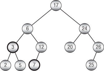
Figure 10.13: You can search a sorted tree from the top down to find lowest common ancestors.
You start at the root, which has value 17. That value is greater than both 3 and 7. Both of those values lie down the left child branch, so that's the branch you follow.
Now you compare the node's value, 6, to 3 and 17. The value 6 is greater than 3 and less than 7, so this is the lowest common ancestor.
The following pseudocode shows this algorithm:
// Find the LCA for the two nodes.TreeNode: FindLcaSortedTree(Integer: value1, Integer: value2)// See if both nodes belong down the same child branch.If ((value1 < Value) && (value2 < Value)) ThenReturn LeftChild.FindLca(value1, value2)End IfIf ((value1 > Value) && (value2 > Value)) ThenReturn RightChild.FindLca(value1, value2)End If// This is the LCA.Return <this node>End FindLcaSortedTree
This algorithm is implemented as a method in the TreeNode class. It compares the current node's value to the two descendant node values. If both of the target values are less than the node's value, then they both lie down the node's left child subtree, so the algorithm recursively calls itself on the left child. Similarly, if both values are greater than the node's value, then they both lie down the node's right child subtree, so the algorithm recursively calls itself on the right child.
If the target values do not both lie down the same child subtree, then either they are in different child subtrees or the current node holds one of the values. In either of those cases, the current node is the lowest common ancestor, so the algorithm returns the current node.
Parent Pointers
Suppose the tree's nodes include references to their parent nodes. In that case, you can use a simple marking strategy to find the lowest common ancestor of two nodes. Follow the parent pointers from the first node to the root marking each node as visited. Then follow parent pointers from the second node to the root until you reach a marked node. The first marked node that you reach is the LCA. Finish by following the parent pointers above the first node again to reset their marked flags so the tree will be ready for future operations.
The following pseudocode shows this algorithm:
TreeNode: FindLcaParentPointers(TreeNode: node1, TreeNode: node2)# Mark nodes above node1.TreeNode: node = node1While (node != null)node.Marked = Truenode = node.ParentEnd While# Search nodes above node2 until we find a marked node.TreeNode: lca = nullnode = node2While (node != null)If (node.Marked) Thenlca = nodeBreakEnd Ifnode = node.Parent# Unmark nodes above node1.node = node1While (node != null)node.Marked = Falsenode = node.ParentEnd While# Return the LCA.Return lcaEnd FindLcaParentPointers
This code simply follows the algorithm described earlier.
This algorithm has the drawback that it requires extra storage for the Marked field in the TreeNode class.
Parents and Depths
If the TreeNode class contains a Depth field that indicates the node's depth in the tree in addition to a parent reference, then you can you can use that field to implement another method for finding the LCA without using marking. Starting at the node with the greater depth, follow parent nodes up the tree until you reach the other node's depth. Then move up both nodes’ parent chains until the two paths meet at the same node. The following pseudocode shows this algorithm:
TreeNode: FindLcaParentsAndDepths(TreeNode: node1, TreeNode: node2)// Climb up until the nodes have the same depth.While (node1.Depth > node2.Depth) node1 = node1.ParentWhile (node2.Depth > node1.Depth) node2 = node2.Parent// Climb up until the nodes match.While (node1 != node2)node1 = node1.Parennode2 = node2.ParentEnd WhileReturn node1FindLcaParentsAndDepths
This algorithm has a couple of advantages over the preceding approach. In this algorithm, the Depth field basically replaces the Marked field, so it doesn't use any extra space. It is slightly faster because it doesn't need to retrace the first node's path to the root to unmark previously marked nodes. It also only traces the paths until they meet, so it doesn't need to go all the way to the root.
The preceding version may still be useful, however, if you want the TreeNode class to have a Marked field for use by some other algorithm.
General Trees
The first LCA algorithm described in this chapter used a top-down search through a sorted binary tree to find the LCA of two nodes. You can also use a top-down approach to find the LCA for two values in an unsorted tree.
The previous algorithm compared the target values at each node to the node's value to see which branch it should move down in its search. Because the tree in the new scenario is unsorted, comparing values won't tell you which branch to move down. Instead, you basically need to perform a search of the complete tree to find the nodes containing the target values. That idea leads to the following straightforward algorithm:
TreeNode: FindLcaExhaustively(Integer: value1, Integer: value2)<Traverse the tree to find the path from the root to value1.><Traverse the tree to find the path from the root to value2.><Follow the two paths until they diverge.><Return the last node that is on both paths.>FindLcaExhaustively
In some sense, this algorithm is optimal. You don't know where the values might be in the tree, so in the worst case you might need to search the entire tree before you find them. If the tree contains N nodes, then this is an O(N) algorithm.
Although you can't change that algorithm's big O run time, you can improve the real-world performance slightly by searching for both values at the same time and stopping when you find the LCA.
The basic idea is similar to the one used by the algorithm for the sorted tree. At each node, you determine down which child branch the two values lie. The LCA is the first node where the values lie down different child branches.
However, because this tree isn't sorted, you can't use the nodes’ values to determine which child subtrees contain them. Instead, you need to perform a traversal of the subtrees, but you need to be careful. If you simply traverse the subtrees at every step, then you will end up traversing the same parts of the tree many times.
For example, suppose that the target values are near the rightmost edge of the tree. At the root node, you would traverse most of the tree before learning that you need to move down to the rightmost child. Then at the root's right child node, you would traverse most of its subtree to learn that you need to move down to its rightmost child. You would repeatedly traverse smaller and smaller pieces of the right part of the tree until you finally reached the LCA.
You can avoid those repeated traversals if you keep track of both values as you traverse the tree only once. The following pseudocode demonstrates that approach:
TreeNode: FindLca(Integer: value1, Integer: value2)Boolean: contains1, contains2Return ContainsNodes(value1, value2,Output contains1, Output contains2)End FindLca
This algorithm simply calls the root node's ContainsNodes algorithm, shown in the following pseudocode, to do all of the actual work:
// Find the LCA for the two nodes.TreeNode: ContainsNodes(Integer: value1, Integer: value2,Output Boolean: contains1, Output Boolean: contains2)// Assume we won't find the target values.contains1 = (Value == value1)contains2 = (Value == value2)If (contains1 && contains2) Then Return <this node>// See which children contain the values.For Each child In Children// Check this child.Boolean: has1, has2TreeNode: lca = child.ContainsNodes(value1, value2,Output has1, Output has2)// If we have found the LCA, return it.If (lca != null) Then Return lca// Update contains1 and contains2.If (has1) Then contains1 = TrueIf (has2) Then contains2 = True// If we found both values in different// children, then this is the LCA.If (contains1 && contains2) Then Return <this node>Next childReturn nullEnd ContainsNodes
This algorithm takes two output parameters that it uses to keep track of whether a particular node's subtree contains the target values. Alternatively, you could make the method return a tuple containing the LCA and those two values instead of using output parameters.
The code first sets the Boolean variables contains1 and contains2 to true if the current node equals either of the target values. If both of those values are true, then the two values are the same and they equal the node's value, so the code returns the node as the LCA.
Next, the code loops through the node's children. It recursively calls the ContainsNodes algorithm to look for the LCA in that child's subtree. The recursive call sets the has1 and has2 variables to indicate whether the subtree contains the target values.
If the recursive call returns an LCA, then the current instance of the algorithm returns it.
Otherwise, if the recursive call returns null, the current instance of the algorithm uses has1 and has2 to update contains1 and contains2. If contains1 and contains2 are now both true, the algorithm returns the current node as the LCA.
If the algorithm finishes examining all of the current node's children without finding the LCA, then the algorithm returns null.
Euler Tours
The previous LCA algorithms use the tree's structure to find the LCA. Other algorithms preprocess the tree to make it easier to find LCAs later. One approach that makes it at least conceptually easier to find LCAs is to look at the tree's Euler tour.
An Euler tour or Eulerian path is a path through a network that crosses every edge once. (Euler is pronounced “oiler.”) To make an Euler tour in a tree, you double each branch so that there is an upward and downward branch. You then traverse the tree as shown in Figure 10.14.

Figure 10.14: This tree's Euler tour visits the nodes in the order 0, 1, 3, 6, 3, 1, 4, 7, 4, 1, 0, 2, 5, 2, 0.
The dashed path in Figure 10.14 shows the Euler tour. Notice that nonleaf nodes are visited multiple times as the path moves up and down the tree. For example, the tour visits node 1 three times: on the way down to node 3, on the way back up from node 3 and down to node 4, and on the way back up from node 4. The complete tour visits the tree's nodes in the order 0, 1, 3, 6, 3, 1, 4, 7, 4, 1, 0, 2, 5, 2, 0.
A useful feature of the Euler tour is that the LCA of two nodes lies between their entries in the tour. For example, consider nodes 3 and 7 in Figure 10.14, and look at their positions in the Euler tour. First, notice that all of node 3s entries in the tour (it appears twice) come before all of node 7s entries in the tour (it appears only once). If you look at the interval between any of node 3s entries and any of node 7s entries, then that interval contains the LCA of nodes 3 and 7. For example, the longest such interval visits the nodes 3, 6, 3, 1, 4, 7 and node 1 is the LCA.
These observations lead to the following high-level steps for finding LCAs.
- Preprocessing:
- Add two new fields to the node class.
Depthis the node's depth in the tree.TourLocationis the index of the node's first position in the Euler tour.
- Perform a traversal of the tree to assign each node's
Depth. - Build the Euler tour and save it as a list containing the nodes in the order in which they are visited. Set each node's
TourLocationvalue to the index of the node's first occurrence in the tour.
- Add two new fields to the node class.
- To find the LCA, loop between the two nodes’
TourLocationvalues to examine the nodes that appear between them in the tour. The node with the smallestDepthis the LCA.
This algorithm requires some preprocessing, but scanning the tour is much easier to understand than the recursive ContainsNode algorithm described in the preceding section. One drawback to this approach is that you need to update the tour information if you modify the tree.
Chapter 14, “More Network Algorithms,” explains how you can find Eulerian paths through a network.
All Pairs
The fastest and easiest possible way to find LCAs would be simply to look up the LCA in an array. For example, the value LCA[i, j] would return the LCA of nodes i and j.
The following pseudocode snippet shows how you might build that array:
// Allocate the array.Lcas = new TreeNode[numNodes, numNodes]// Fill in the array values.For i = 0 to <number of nodes – 1>For j = i to <number of nodes – 1>Lcas[i, j] = FindLca(i, j)Lcas[j, i] = Lcas[i, j]Next jNext i
This code allocates the array and then loops through all of the pairs of node values. For each pair, it uses some other method such as the Euler tour to find the LCA and saves the result in the array.
Building the array requires you to examine ![]() pairs of nodes, so it is relatively slow. The array also uses
pairs of nodes, so it is relatively slow. The array also uses ![]() memory, so it takes up a lot of space. You will also need to restructure or rebuild the array if you modify the tree. All of those factors make this method impractical for large trees.
memory, so it takes up a lot of space. You will also need to restructure or rebuild the array if you modify the tree. All of those factors make this method impractical for large trees.
The key to the Euler Tour approach is finding the minimum depth of the nodes within a range of values given by part of the Euler tour. The general problem of finding the minimum value in a range of values such as this is called the range minimum query problem. Other versions of this algorithm use special techniques to solve the range minimum query problem quickly. They allow the algorithm to find LCAs in constant time with only O(N) amount of extra storage. Unfortunately, those algorithms are too complicated to include here.
Threaded Trees
A thread is a sequence of links that allows you to move through the nodes in a tree or network in a way other than by following normal branches or links. A threaded tree is a tree that contains one or more threads.
For example, Figure 10.15 shows a tree with threads represented by dashed arrows.

Figure 10.15: A threaded tree contains references that let you move through the tree without following its normal branches.
The threads shown in Figure 10.15 point from a node to the nodes that come before and after it in an inorder traversal. The first and last threads shown in Figure 10.15 don't have nodes to point to, so they are set to null. The threads allow an algorithm to perform an inorder traversal or reverse traversal more quickly than is possible by using the branches alone.
To use this kind of threaded tree, you need to know two things: how to build the tree and how to traverse it.
Building Threaded Trees
A threaded tree starts with a single node that has no branches and with threads set to null. Creating that node is simple.
The trick is adding new nodes to the tree. There are two cases, depending on whether you add a new node as the left or right child of its parent.
First, suppose that you're adding the new node as a left child. Suppose that you're adding the node 3 as the left child of node 4 in the tree shown in Figure 10.15.
Because of where the new node is placed, its value is the next smaller value compared to its parent's value. (In this example, 3 is the next smaller value before 4.) That means the node before the new one in the traversal is the node that was formerly the node before the parent. In this example, the node before 3 is the node that was before 4—in this case, 2. When creating the new node, set the new node's left thread equal to the value of the parent's left thread.
The parent's predecessor in the traversal is now the new node. The parent's left branch points to the new node, so the parent no longer needs its left thread and you should set it equal to null.
The new node's right thread should point to the next node in the tree's traversal. Because of where the new node is placed, that is the parent node, so you should set the new node's right thread to its parent. In this example, node 3's right thread should point to node 4. The parent's right child link or right thread is still correct, so you don't change it.
Figure 10.16 shows the updated tree with node 3 added.

Figure 10.16: When you insert a node as a left child, its left thread points where the parent's left thread used to point.
When you add a node as the right child of an existing node, the steps are similar, with the roles of the left and right branches and threads reversed. The new node's right thread takes the value that the parent's right thread had, and the parent's right thread is set to null. The new node's left thread points to the parent node.
Figure 10.17 shows the tree in Figure 10.16 with the new node 8 inserted.

Figure 10.17: When you insert a node as a right child, its right thread points where the parent's right thread used to point.
The following pseudocode shows an algorithm for inserting a node into a threaded sorted tree:
// Add a node to this node's sorted subtree.AddNode(Data: new_value)// See if the new value is smaller than ours.If (new_value < this.Value)// The new value is smaller. Add it to the left subtree.If (this.LeftChild != null)Then this.LeftChild.AddNode(new_value)Else// Add the new child here.ThreadedNode child = new ThreadedNode(new_value)child.LeftThread = this.LeftThreadchild.RightThread = thisthis.LeftChild = childthis.LeftThread = nullEnd IfElse// The new value is not smaller. Add it to the right subtree.If (this.RightChild != null)Then this.RightChild.AddNode(new_value)Else// Add the new child here.ThreadedNode child = new ThreadedNode(new_value)child.LeftThread = thischild.RightThread = this.RightThreadthis.RightChild = childthis.RightThread = nullEnd IfEnd IfEnd AddNode
The algorithm first compares the new value to the node's value. If the new value is smaller, the algorithm adds it to the left subtree.
If the node has a left child, the algorithm recursively calls its AddNode method.
If the node has no left child, the algorithm adds the new node here. It creates the new node, sets its left thread equal to the current node's left thread, and sets its right thread equal to the current node. It sets the current node's left branch to point to the new node and sets the current node's left thread to null.
If the new value is greater than or equal to the current node's value, the algorithm performs similar steps to place the new value in the right subtree. The steps are the same as the case when the new value is smaller than the current node's value, with the roles of the left and right branches and threads reversed.
This algorithm is similar to the previous algorithm for adding a node to a sorted tree. Both versions recursively search down through the tree to find the new node's location. The only difference is that this version takes extra action to sort out threads when it finally creates the new node.
As with the previous version, if you use this method to build a threaded sorted tree containing N nodes, this algorithm takes ![]() time if the values are initially arranged randomly. The algorithm takes
time if the values are initially arranged randomly. The algorithm takes ![]() time in the worst case when the values are initially sorted or sorted in reverse order.
time in the worst case when the values are initially sorted or sorted in reverse order.
Using Threaded Trees
The following pseudocode uses threads to perform an inorder traversal:
InorderWithThreads(BinaryNode: root)// Start at the root.BinaryNode: node = root// Remember whether we got to a node via a branch or thread.// Pretend we go to the root via a branch so we go left next.Boolean: via_branch = True// Repeat until the traversal is done.While (node != null)// If we got here via a branch, go// down and to the left as far as possible.If (via_branch) ThenWhile (node.LeftChild != null)node = node.LeftChildEnd WhileEnd If// Process this node.<Process node>// Find the next node to process.If (node.RightChild == null) Then// Use the thread.node = node.RightThreadvia_branch = FalseElse// Use the right branch.node = node.RightChildvia_branch = TrueEnd IfEnd WhileEnd InorderWithThreads
The algorithm starts by initializing the variable node to the root node. It also initializes the variable via_branch to True to indicate that the algorithm got to the current node via a branch. Treating the root node in this way makes the algorithm move to the leftmost node in the tree in the next step.
The algorithm then enters a loop that continues until the variable node drops off the tree at the end of the traversal.
If the algorithm got to the current node via a branch, it should not necessarily process that node just yet. If that node has a left branch, the nodes down that subtree have values smaller than the current node, so the algorithm must visit them first. To do that, the algorithm moves as far down the left branches as possible. For example, in Figure 10.15 this occurs when the algorithm moves from node 6 to node 9. The algorithm must first move down to node 7 before it processes node 9.
The algorithm then processes the current node.
Next, if the node's right branch is null, the algorithm follows the node's right thread. If the right thread is also null, the algorithm sets node to null and the While loop ends.
If the node does have a right thread, the algorithm sets via_branch to False to indicate that it got to the new node via a thread, not a branch. In Figure 10.15, this happens several times, such as when the algorithm moves from node 4 to node 5. Because via_branch is False, the algorithm will process node 5 next.
If the current node's right branch is not null, the algorithm follows it and sets via_branch to True so that it moves down that node's left subtree during the next trip through the While loop.
The following list describes the steps taken by this algorithm to traverse the tree shown in Figure 10.15:
- Start at the root, and set
via_branchtoTrue. - Variable
via_branchisTrue, so follow the left branches to 2 and then 1. Process node 1. - Follow the right thread to 2, and set
via_branchtoFalse. - Variable
via_branchisFalse, so process node 2. - Follow the right branch to 4, and set
via_branchtoTrue. - Variable
via_branchisTrue, so try to move down the left branches. There is no left branch here, so stay at node 4 and process node 4. - Follow the right thread to 5 and set
via_branchtoFalse. - Variable
via_branchisFalse, so process node 5. - Follow the right branch to 6, and set
via_branchtoTrue. - Variable
via_branchisTrue, so try to move down the left branches. There is no left branch here, so stay at node 6 and process node 6. - Follow the right branch to 9, and set
via_branchtoTrue. - Variable
via_branchisTrue, so follow the left branch to 7 and process node 7. - Follow the right thread to 9, and set
via_branchtoFalse. - Variable
via_branchisFalse, so process node 9. - Follow the right thread to
null, and setvia_branchtoFalse. - Variable
nodeis nownull, so theWhileloop ends.
This algorithm still follows all of the nodes’ branches, and it visits every node, so it has run time O(N). However, it doesn't need to let recursive calls unwind back up the child branches, so it saves a bit of time over a normal traversal. It also doesn't use recursion, so it doesn't have problems with deep levels of recursion. It also doesn't need any extra storage space, unlike a breadth-first traversal.
Specialized Tree Algorithms
Over the years, programmers have developed many specialized tree algorithms to solve specific problems. This chapter can't possibly describe every algorithm, but the following sections describe four algorithms that are particularly interesting. They demonstrate the useful techniques of updating a tree to include new data, evaluating recursive expressions, and subdividing geometric areas. The final section explains tries, which are well-known in algorithmic studies.
The Animal Game
In the animal game, the user thinks of an animal. The program's simple artificial intelligence tries to guess what it is. The program is a learning system, so over time it gets better at guessing the user's animal.
The program stores information about animals in a binary tree. Each internal node holds a yes-or-no question that guides the program down the left or right branch. Leaf nodes represent specific animals.
The program asks the questions at each of the nodes that it visits and follows the appropriate branch until it reaches a leaf node where it guesses that node's animal.
If the program is wrong, it asks the user to type a question that it can ask to differentiate between the animal it guessed and the correct answer. It adds a new internal node containing the question and gives that node leaves holding the correct and incorrect animals.
Figure 10.18 shows a small knowledge tree for the game.

Figure 10.18: This knowledge tree can differentiate among dog, cat, fish, snake, and bird.
For example, suppose that the user is thinking about a snake. Table 10.2 shows the questions that the program asks and the answers the user gives.
Table 10.2: The Animal Game Trying to Guess Snake
| THE PROGRAM ASKS: | THE USER ANSWERS: |
| Is it a mammal? | No |
| Does it have scales? | Yes |
| Does it breathe water? | No |
| Is it a snake? | Yes |
For another example, suppose that the user is thinking about a giraffe. Table 10.3 shows the questions the program asks and the answers the user gives in this example.
Table 10.3: The Animal Game Trying to Guess Giraffe
| THE PROGRAM ASKS: | THE USER ANSWERS: |
| Is it a mammal? | Yes |
| Does it bark? | No |
| Is it a cat? | No |
| What is your animal? | Giraffe |
| What question could I ask to differentiate between a cat and a giraffe? | Does it have a long neck? |
| Is the answer to this question true for a giraffe? | Yes |
The program then updates its knowledge tree to hold the new question and animal. The new tree is shown in Figure 10.19.

Figure 10.19: This knowledge tree can now differentiate between cat and giraffe.
Expression Evaluation
You can model many situations with trees. You can model mathematical expressions by creating an internal node for each operator and a leaf node for each numeric value.
Mathematical expressions naturally break into subexpressions that you must evaluate before you can evaluate the expression as a whole. For example, consider the expression ![]() . To evaluate this expression, you must first evaluate
. To evaluate this expression, you must first evaluate ![]() and
and ![]() . You can then divide the results of those calculations to get the final result.
. You can then divide the results of those calculations to get the final result.
To model this expression as a tree, you build subtrees to represent the subexpressions. You then join the subtrees with a parent node that represents the operation that combines the subexpressions—in this case, division.
Figure 10.20 shows the tree representing the expression ![]() .
.

Figure 10.20: You can use trees to evaluate mathematical expressions.
Each internal node has children representing its operands. For example, binary operators such as + and / have left and right children, and the operator must combine the children's values.
You can think of the leaf nodes as special operators that convert a text value into a numeric one. In that case, the leaf nodes must hold their text.
The only thing missing from the arithmetic node class is a method to evaluate the node. That method should examine the type of node and then return an appropriate result. For example, if the operator is +, the method should recursively make its operands evaluate their subexpressions, and then it can add the results.
The following pseudocode creates an enumeration that defines values that indicate a node's operator type:
Enumeration OperatorsLiteralPlusMinusTimesDivideNegateEnd Enumeration
This enumeration defines operator types for literal values such as 8, addition, subtraction, multiplication, division, and unary negation (as in ![]() ). You can add other operators such as square root, exponentiation, sine, cosine, and others.
). You can add other operators such as square root, exponentiation, sine, cosine, and others.
The following pseudocode shows an ExpressionNode class that represents a node in a mathematical expression tree:
Class ExpressionNodeOperators: OperatorExpressionNode: LeftOperand, RightOperandString: LiteralText// Evaluate the expression.Float: Evaluate()Case OperatorLiteral:Return Float.Parse(LiteralText)Plus:Return LeftOperand.Evaluate() + RightOperand.Evaluate()Minus:Return LeftOperand.Evaluate() - RightOperand.Evaluate()Times:Return LeftOperand.Evaluate() * RightOperand.Evaluate()Divide:Return LeftOperand.Evaluate() / RightOperand.Evaluate()Negate:Return -LeftOperand.Evaluate()End CaseEnd EvaluateEnd ExpressionNode
The class begins by declaring its properties. The Operator property is a value from the Operators enumerated type.
The LeftOperand and RightOperand properties hold links to the node's left and right children. If the node represents a unary operator such as negation, only the left child is used. If the node represents a literal value, neither child is used.
The LiteralText property is used only by literal nodes. For a literal node, it contains the node's textual value, such as 12.
The Evaluate method examines the node's Operator property and takes appropriate action. For example, if Operator is Plus, the method calls the Evaluate method for its left and right children, adds their results, and returns the sum.
After you build an expression tree, evaluating it is easy. You simply call the root node's Evaluate method.
The hardest part of evaluating mathematical expressions is building the expression tree from a string such as ![]() . That is a string operation, not a tree operation, so this topic is deferred until Chapter 15, which covers strings in depth.
. That is a string operation, not a tree operation, so this topic is deferred until Chapter 15, which covers strings in depth.
Interval Trees
Suppose that you have a collection of intervals with start and end points in a one-dimensional coordinate system. For example, if the intervals represent time spans, then their end points would be start and stop times. An appointment calendar application might need to search a collection of intervals to see whether a new appointment overlaps any existing appointment.
You can think of each interval as representing a range of values ![]() on the x-axis. After you have the intervals, you might want to find those that include a specific x-coordinate.
on the x-axis. After you have the intervals, you might want to find those that include a specific x-coordinate.
One approach to this problem would be simply to loop through the intervals and find those that include the target value. If there are N intervals, then that would take O(N) steps.
An interval tree is a data structure that makes this kind of lookup faster. Each node in an interval tree represents a single midpoint coordinate. The node holds two child pointers, one leading to intervals that lie entirely to the left of the midpoint and one leading to intervals that lie entirely to the right of the midpoint. The node also includes two lists of the intervals that surround the midpoint. One of those lists is sorted by their left end coordinates, and the other is sorted by their right end coordinates.
For example, consider the segments shown in Figure 10.21. The dark horizontal lines represent the intervals. (Ignore their y-coordinates.) The gray dots represent nodes in the interval tree. The vertical gray lines show which intervals surround the centers of the nodes.

Figure 10.21: Horizontal lines represent intervals. Vertical lines show which intervals surround the tree nodes.
Figure 10.22 shows a representation of this tree's root node.

Figure 10.22: Interval tree nodes contain lists of overlapping intervals sorted by their left and right edges.
The node includes links to child nodes, plus two lists holding nodes that overlap with the node's midpoint. The left overlap list holds the intervals sorted by their left end points. The right overlap list holds the intervals sorted by their right end points. For example, the first interval in the right overlap list has a larger right coordinate than the other two intervals in that list.
The following sections explain how to build and use an interval tree.
Building the Tree
The following code snippet shows how you could define an Interval class to represent an interval:
Class IntervalInteger: LeftCoordinate, RightCoordinateConstructor(Integer: coordinate1, Integer: coordinate2)// Save the points in order.If (coordinate1.X < coordinate2.X) ThenLeftCoordinate = coordinate1RightCoordinate = coordinate2ElseLeftCoordinate = coordinate2RightCoordinate = coordinate1End IfEnd ConstructorEnd Class
The Interval class simply stores the interval's coordinates. Its constructor saves the new interval's coordinates where LeftCoordinate is smaller than RightCoordinate.
The following code snippet shows how you could define the IntervalNode class's fields:
Class IntervalNodeFloat: Min, Mid, MaxList<Interval>: LeftOverlap = New List<Interval>List<Interval>: RightOverlap = New List<Interval>IntervalNode: LeftChild = nullIntervalNode: RightChild = nullConstructor(Float: xmin, Float: xmax)Xmin = xminXmax = xmaxXmid = (xmin + xmax) / 2End Constructor…End Class
For convenience, the node stores the minimum, maximum, and middle coordinates of the area that it represents. The constructor stores the minimum and maximum values and calculates the middle value.
To build an interval tree, start with a root node and then add the intervals to it. The following pseudocode shows the IntervalNode class's AddInterval method, which adds a new interval to the node:
// Add an interval to the node.AddInterval(Interval: interval)If <interval lies to the left of Mid>If LeftChild == null Then <Create LeftChild>LeftChild.AddInterval(interval)Else If <interval lies to the right of Mid>If RightChild == null Then <Create RightChild>RightChild.AddInterval(interval)Else<Add interval to left overlap list><Add interval to right overlap list>End IfEnd AddInterval
This method compares the new interval's coordinates to the node's Mid value. If the interval lies completely to the left of the node's Mid value, then the method adds the interval to the left child node. If the interval lies to the right of the node's Mid value, then the method adds the interval to the right child node.
If the interval spans the Mid value, then the method adds it to the node's left and right overlap lists. You can either add the interval to the lists in sorted order now or wait until the tree is finished and then sort the lists in ![]() time, where K is the number of items in the lists.
time, where K is the number of items in the lists.
Intersecting with Points
The following pseudocode shows how an interval tree can search for intervals that contain a target coordinate value:
FindOverlappingIntervals(List<Interval>: results,Integer: target)// Check our overlap intervals.If (target <= Mid) Then<Search the left overlap list>Else<Search the right overlap list>End If// Check the children.If ((target < Mid) And (LeftChild != null)) ThenLeftChild.FindOverlappingIntervals(results, target)Else If ((target > Mid) And (RightChild != null)) ThenRightChild.FindOverlappingIntervals(results, target)End IfEnd FindOverlappingIntervals
This method takes as inputs a result list that will hold any intervals that intersect with the target coordinate and the target coordinate. It first checks the node's overlap lists to see whether any of the intervals in the lists contain the target value. The fact that the overlap lists are sorted makes searching them a bit easier.
For example, if target < Mid, then the method searches its left overlap list. The intervals in that list have RightCoordinate >= Mid, so an interval contains the target value if LeftCoordinate <= target. Because the intervals are sorted by increasing LeftCoordinate value, you only need to search the list until you find an interval with LeftCoordinate > target. Then you know that the later intervals also have LeftCoordinate > target, so they cannot contain the target value.
The same logic applies in reverse for the right overlap list.
After the method has searched the overlap lists for the target value, it recursively calls itself for the left or right child node as appropriate.
Intersecting with Intervals
The preceding section explained how you can search an interval tree to find intervals that overlap a target point. You can also use a recursive search to find intervals that overlap a target interval. Simply traverse the tree as before, this time examining any node that might overlap the target interval. The following pseudocode shows this technique:
FindOverlappingIntervals(List<Interval>: results,Integer: xmin, Integer: xmax)// Check our overlap intervals.If (xmax <= Mid) Then<Search the left overlap list>Else if (xmin >= Mid) Then<Search the right overlap list>Else<Add all node intervals to the results>End If// Check the children.If ((xmin < Mid) && (LeftChild != null)) ThenLeftChild.FindOverlappingIntervals(results, xmin, xmax);End IfIf ((xmax > Mid) && (RightChild != null)) ThenRightChild.FindOverlappingIntervals(results, xmin, xmax);End IfEnd FindOverlappingIntervals
The xmin and xmax parameters give the target interval's minimum and maximum coordinates. The algorithm first uses those values to decide whether its intervals might intersect the target interval.
If xmax <= Mid, then the target interval lies to the left of the node's midpoint. In that case, the method searches the node's left overlap list. If any of those intervals has left coordinate larger than the target interval's maximum coordinate, then that interval and those that come after it in the list are completely to the right of the target interval, so they do not overlap with it. That means the algorithm can break out of its loop and stop searching the left overlap list.
Figure 10.23 shows a left overlap list. The dark horizontal lines represent intervals in the tree. Recall that they are arranged in order of increasing left coordinate. The gray line in the upper left is the target interval. The dashed lines show the edges of that interval. The algorithm only needs to search through the list's intervals until it reaches one with left coordinate greater than the target interval's right coordinate. In Figure 10.23, the list's second-to-last interval lies to the right of the target interval, so the algorithm doesn't need to check the list further.

Figure 10.23: The algorithm only needs to check the left overlap list until it finds an interval with left coordinate greater than the target interval's right coordinate.
The same steps apply in reverse to the node's right intervals. If xmin >= Mid, then the target interval lies to the right of the node's midpoint. In that case, the method searches the node's right overlap list.
If neither of the previous two conditions is true, then the target interval spans the node's midpoint, so the algorithm adds all of its intervals to the results list.
After searching the node's overlap list, the algorithm considers its child subtrees. If the target interval's left coordinate is less than the node's midpoint, then it is possible that the left subtree might contain intervals that overlap with the target. In that case, the algorithm calls itself recursively to examine the left subtree.
Similarly, if the target interval's right coordinate is greater than the node's midpoint, then the algorithm recursively examines the node's right subtree.
One of the larger differences between this algorithm and the previous one that searched for intervals that overlap a point is in these recursive calls. Because the target point could not lie both to the left and the right of a node's midpoint, the previous algorithm needed to search only one of the node's subtrees. In contrast, a target interval can be both to the left and the right of the midpoint, so the new algorithm might search both child subtrees.
Quadtrees
Quadtrees are tree data structures that help locate objects in two-dimensional space. For example, suppose you have an application that displays several thousand delivery locations. If the user clicks the map, the program needs to search through all of the locations to find the one closest to where the user clicked. If the locations are stored in a simple list, the program must perform a sequential search to find the closest point. A quadtree can make the search much faster.
In a quadtree, a node represents a rectangle in two-dimensional space. The node contains a list of items that are contained within its rectangle.
If a quadtree node contains more than a predetermined number of items, it is split into four child nodes representing the parent node's northwest, northeast, southeast, and southwest quadrants. The items are then moved into the appropriate child nodes.
To use a quadtree to find an item with given x- and y-coordinates, you start at the root node. If the quadtree node has children, you use the item's coordinates to determine which child contains the item. You then recursively search that child for the item. If you reach a node that doesn't have children, you search the items it contains for an item at the target location.
To see why this makes the search faster, suppose that the mapping application described a moment ago contains a list of 1,500 locations. Searching that list linearly will require on average roughly 750 comparisons.
In contrast, suppose that you store the items in a quadtree where each node can hold at most 100 items. If the nodes are reasonably evenly distributed around the map, the quadtree would logically look like the one shown in Figure 10.24.

Figure 10.24: If each leaf node can hold 100 items and the items are evenly distributed, this quadtree can hold roughly 1,600 items.
The root node's area is divided into four quadrants, each of which is divided into four smaller quadrants. Each leaf node representing a smaller quadrant can hold up to 100 items. Its parent node holds four leaf nodes, so it contains up to 400 items. The root node holds four of those nodes, so the whole tree can contain up to 1,600 items.
To find the item that the user clicked in this quadtree, you need to determine which larger quadrant contains the item and then which smaller quadrant within the larger quadrant contains the item. Then you need to search up to 100 items in the leaf node. The result is an average of two quadrant tests plus roughly 50 item tests. The relative speed of the quadrant tests and item tests may vary depending on your implementation, but the speed is generally much faster than the 750 item tests required by a simple list.
If a quadtree contains N nodes, each of which can hold up to K items, and the items are distributed reasonably evenly in the map area, the tree has a height of roughly ![]() . In the previous example,
. In the previous example, ![]() and
and ![]() , so the height should be roughly
, so the height should be roughly ![]() , which is close to the height of 2 for the tree shown in Figure 10.24.
, which is close to the height of 2 for the tree shown in Figure 10.24.
Figure 10.25 shows another way to visualize a quadtree. In this figure, the quadtree contains 200 items, and each quadtree node can hold at most 10 items. (In a real program, you would probably want to let each node hold more items so that they don't split as often.) The program draws a box around each quadtree node so that you can see how the area is divided.

Figure 10.25: Each box shows a quadtree node's area.
In the tree shown in Figure 10.25, the full map area is divided into four quadrants, and each of these is divided into smaller quadrants. Some of the smaller quadrants are divided again, and some of those areas are divided one last time.
To manage a quadtree, you need algorithms to add a new item to a subtree and to find an item in a subtree. You may also want an algorithm to draw the items, as shown in Figure 10.25.
The following pseudocode shows the basic class definition for a quadtree node:
Class QuadtreeNode// The maximum number of points allowed in a quadtree node.Integer: MaxItems = 10// The items in this quadtree node.List Of Data: Items// The area's bounds and middle X and Y values.Float: Xmin, Ymin, Xmid, Ymid, Xmax, Ymax// The child quadtree nodes in order NW, NE, SW, SE.QuadtreeNode: Children[]// Initializing constructor.Constructor(Float: xmin, Float: ymin, Float: xmax, Float: ymax)Xmin = xminYmin = yminXmax = xmaxYmax = ymaxXmid = (xmin + xmax) / 2Ymid = (ymin + ymax) / 2End ConstructorEnd QuadtreeNode
The value MaxItems indicates the maximum number of items a node can hold before it must be split into quadrants.
The Items property contains the items that the node holds. If the node is internal, Items is null, and the items are stored in the node's child subtrees.
The Xmin, Ymin, Xmax, and Ymax values store the bounds of the area represented by the node. The Xmid and Ymid values give the middle X and Y coordinates of the area. These are used to determine which quadrant contains an item.
This class provides a constructor that initializes the node's bounds and the Xmid and Ymid properties. You could calculate Xmid and Ymid whenever you need them, but those values are used frequently (at least for nonleaf nodes), so you can save time by initializing them now.
The following sections explain how to add items to a quadtree and how to find items in a quadtree.
Adding Items
The following pseudocode shows how a QuadtreeNode can add a new item to its subtree:
// Add an item to this node.AddItem(Item: new_item)// See if this quadtree node is full.If ((Items != null) And (Items.Count >= MaxItems)) Then// Divide this quadtree node.Children.Add(new QuadtreeNode(Xmin, Ymin, Xmid, Ymid)) // NWChildren.Add(new QuadtreeNode(Xmid, Ymin, Xmax, Ymid)) // NEChildren.Add(new QuadtreeNode(Xmin, Ymid, Xmid, Ymax)) // SWChildren.Add(new QuadtreeNode(Xmid, Ymid, Xmax, Ymax)) // SE// Move the points into the appropriate subtrees.For Each item in ItemsAddItemToChild(point)Next item// Remove this node's points list.Points = nullEnd If// Add the new item here or in the appropriate subtree.If (Items != null)Items.Add(new_item)ElseAddItemToChild(new_item)End IfEnd AddItem
If the current node is a leaf node and adding one more item would give it too many items, the algorithm splits the node by creating four child nodes. It then loops through the items and calls the AddItemToChild method described shortly to move each item into the appropriate child subtree. It then sets the Items list to null to indicate that this is an internal node.
After splitting the node if necessary, the algorithm adds the new item. If the Items property is not null, then this is a leaf node, so the algorithm adds the new item to the Items list.
If the Items property is null, then this is an internal node. In that case, the algorithm calls the AddItemToChild method described next to move each item into the appropriate child subtree.
The following pseudocode shows the AddItemToChild method:
// Add an item to the appropriate child subtree.AddItemToChild(Item: new_item)For Each child in ChildrenIf ((new_item.X >= child.Xmin) And(new_item.X <= child.Xmax) And(new_item.Y >= child.Ymin) And(new_item.Y <= child.Ymax))Thenchild.AddItem(new_item)BreakEnd IfNext childEnd AddItemToChild
This algorithm loops through the node's children. When it finds the child with bounds that include the new item's location, it calls the child's AddItem method described earlier to add the new item to that child.
Finding Items
You can probably imagine how to use quadtree to find the item at a specific point. Starting at the root node, you determine which child node contains the target point. You then recursively search that child for the item.
That almost works, but there's a catch. Suppose that you want to find the item closest to a target point, but that point lies close to the edge between two quadtree nodes. In that case, the closest item might lie in the quadtree node that does not contain the target point.
Furthermore, the objects stored in the quadtree might not be simple points. They may be bigger objects such as circles, line segments, and polygons. In that case, where should you store an item that straddles the edges between two or more quadtree nodes?
One approach is to store the item in every quadtree node that overlaps the object so that the algorithm can find it no matter which area the user clicks. If you use this approach, you need to change the algorithms to work with two-dimensional items. For example, the search algorithm cannot simply compare the target point to the item's location. Instead, it must use some method to see whether the target point lies within the item.
One problem with this approach is that it requires duplicate items representing the same object in different quadtree nodes. That wastes space and fills quadtree nodes sooner than they would be filled otherwise, so they must split more often and that makes the tree deeper.
Another approach is to represent each item with a specific point, perhaps in its center or upper-left corner. Then, when you need to find an item, you search quadtree nodes with areas that overlap an area around the target point that is big enough to include the largest possible item.
For example, the program shown in Figure 10.25 stores circles with radius 5 that are represented by their center points. When searching for an item at location (A, B), the program examines any quadtree node with an area that intersects the rectangle ![]() and
and ![]() .
.
The changes to the algorithms aren't too complicated, but they make the code quite a bit longer.
Tries
A trie (the word comes from “retrieval” but is usually pronounced “try”) is a tree that holds strings. Each internal node represents a single letter. Leaf nodes may represent more than one letter. A path from the root to a leaf node corresponds to a string.
A partial path from the root to an internal node forms a prefix for longer paths, so tries are sometimes called prefix trees.
A path that represents a key string, whether it ends at an internal node or at a leaf node, has an associated value.
Figure 10.26 shows a trie that holds the keys and values shown in Table 10.4.

Figure 10.26: A path through a trie defines a string.
Table 10.4: Keys and Values for the Example Trie
| KEY | VALUE |
| WANE | 29 |
| WISP | 72 |
| WANT | 36 |
For example, consider the path from the root to the node E. The nodes visited correspond to the letters W, A, N, and E, so that node represents the key WANE. That key's value is 29.
For another example, consider the path to the node T. The nodes visited correspond to the letters W, A, N, and T, so the node represents the key WANT. That key's value is 36.
Notice that the path to the node N forms the string WAN, which is a prefix of both WANE and WANT.
Notice also that a leaf node may represent more than one letter. In this example, the node ISP represents three letters. The path from the root to that node represents the key WISP and has value 72.
To add a new key to the trie, you use the key's letters to follow the appropriate path through the trie. If you reach a leaf node and the key has still more letters that are not represented by the current path, you add a new child node to represent the rest of the key.
For example, suppose that you want to add the key WANTED to the trie. You follow the path through the nodes W, A, N, and T. The key still has the letters ED, so you add a new node to hold them. Figure 10.27 shows the new trie.

Figure 10.27: To add a key that is longer than the corresponding path through the tree, add a new leaf node.
Sometimes, when you add a new key to the trie, you find it early. For example, the trie shown in Figure 10.27 already has the nodes needed to represent the key WAN. In that case, all that you need to do is to add a value to the appropriate node, as shown in Figure 10.28.

Figure 10.28: If a trie already contains nodes to represent a key, simply add a value to the key's final node.
Instead of storing a letter in each internal node, you can figure out the node's letter by keeping track of the path you took from the root to get there. For example, you could store a node's children in an array where Children[0] is the branch for the letter A, Children[1] is the branch for the letter B, and so forth.
Figure 10.29 shows the trie from Figure 10.28 with internal node letters moved to the branches. Notice that the node with value 29 doesn't need any extra information because the key it represents is fully specified by the path to the node. In contrast, the path to the node with value 10 specifies only the letters W, A, N, T, and E, so the node needs to store the final D.

Figure 10.29: Instead of storing an internal node's letter in the node, you can figure out the node from the path to the node.
The following two sections explain how you can add items to a trie and find items in a trie.
Adding Items
The following pseudocode shows how you can add an item to a trie. In this code, the phrase remaining node key means part of a key stored in a leaf node, such as D and SP in Figure 10.29.
AddValue(string new_key, string new_value)<If new_key is not blank and matches the remaining node key,place the value in this node and return.><If new_key is blank and the remaining node key is too,place the value here and return.><If new_key is blank but the node's remaining key isn't blank,move the node's remaining key (minus the first letter) intoa child, place the value here, and return.>// If we get to this point, we need a child node.If <The Children array is null> Then// Make the Children array.Children = New TrieNode[26]<If the node's remaining key is not blank,move it into the appropriate child.>End If// Convert the letter into an integer by "subtracting" A.Integer: index = new_key[0] - 'A'// Search the appropriate subtrie.If (Children[index] == null)// This child doesn't exist. Make it and// let it represent the rest of the new key.Children[index] = New TrieNode()Children[index].RemainingKey = new_key.Substring(1)Children[index].Value = new_valueReturnEnd If// Search the appropriate subtrie.Children[index].AddValue(new_key.Substring(1), new_value)End AddValue
This is a fairly confusing algorithm. It may be easier to understand if you draw a tree and then walk through the algorithm, updating it in various ways.
As the algorithm moves through the trie, it removes the letters from the new key corresponding to the branches it crosses. The body of the algorithm then considers the current value of the new key.
First, if the new key is not blank and it matches the remaining node key, the algorithm places the new value in the current node. This would happen in Figure 10.29 if you were setting the value for WANTED. When the algorithm reached the node labeled D, the new key value will be D, and the node's remaining key is D.
Next, if the new key is blank and the node's remaining key is too, the algorithm places the value in this node. This occurs if you set the value of WAN in Figure 10.29. When the algorithm crosses the N branch, the new key is reduced to an empty string. The node at the end of that branch doesn't have any remaining key (only leaf nodes can have remaining key values), so this is where the value for WAN belongs.
Next, if the new key is blank but the node's remaining key isn't, the algorithm moves the node's remaining key into a child. This would happen if the trie contains WANE and WANTED but not WANT. In that case, the path for WANTED will be W, A, N, T, ED. When you add WANT and cross the T branch, the new key value is blank because the path represents the entire new key WANT. But that node has value ED. The algorithm moves the ED down to a child, creating a new E branch and a new node with D as its remaining key.
If the algorithm gets past all of the previous steps, the algorithm must move into a child node's subtrie. Before it tries to do that, it determines whether the node's Children array has been initialized. If it has not, the algorithm creates the array. If the node's remaining key is not blank, the algorithm also moves the remaining key (minus its first letter) into the appropriate child.
The algorithm then examines the child that should contain the new key. If that child doesn't exist, the algorithm creates it and stores the rest of the new key and the new value in it.
If that child does exist, the algorithm recursively calls itself to add the new key (minus its first letter) to that child's subtrie.
Finding Items
A search for a value in a trie follows the same path through the trie but uses a much simpler algorithm because there are fewer special cases to consider. The following pseudocode shows how a search algorithm might work in a trie:
// Find a value in this node's subtrie.Data: FindValue(String: target_key)// If the remaining key matches the// remaining node key, return this node's value.If (target_key == RemainingKey) Then Return Value// Search the appropriate child.If (Children == null) Then Return nullInteger: index = target_key[0] - 'A'If (Children[index] == null) Then Return nullReturn Children[index].FindValue(target_key.Substring(1))End FindValue
The algorithm first compares the target key to the node's remaining key value. If these are the same, two things may have happened. First, the algorithm may have used up the target key and reached a node that doesn't have a remaining value. (This happens if you search for WAN in Figure 10.28.) Second, the algorithm may have reached a node where the remaining target key matches the node's remaining key. (This happens if you search for WANTED in Figure 10.28.) In either case, this code matches the target key, so the algorithm returns its value.
If the remaining target key doesn't match the node's remaining key, the algorithm must search a child node. If the current node has no children, then the target key isn't in the trie, so the algorithm returns null.
If the node has children, the algorithm calculates the index of the target key's child. If that child doesn't exist, the target key isn't in the trie, so the algorithm again returns null.
Finally, if the target key's child exists, the algorithm calls itself recursively for that child to find the target key (minus its first letter).
Summary
Trees can be useful for storing and manipulating hierarchical data. After you build a tree, you can enumerate its values in different orders and search for values within the tree.
The performance of many tree algorithms is related to the tree's height. If a tree holding N nodes is relatively short and wide, its height is ![]() , and those algorithms are fairly quick. If the tree is tall and thin, it could have height O(N), and some of those algorithms perform badly. For example, building a sorted binary tree takes
, and those algorithms are fairly quick. If the tree is tall and thin, it could have height O(N), and some of those algorithms perform badly. For example, building a sorted binary tree takes ![]() time in the best case and
time in the best case and ![]() time in the worst case.
time in the worst case.
Because a tree's height is important to these algorithms, special trees have been devised that rebalance themselves so that they cannot grow too tall and thin. The next chapter describes several kinds of balanced trees, including the B-trees and B+trees used by many database systems to store and search indices efficiently.
Exercises
You can find the answers to these exercises in Appendix B. Asterisks indicate particularly difficult problems. Two asterisks indicate extremely difficult or time-consuming problems.
- Can a perfect binary tree hold an even number of nodes?
- A perfect tree is full and complete, although not all full and complete trees are perfect. Draw a tree that is full and complete but not perfect.
- Use induction to prove that the number of branches B in a binary tree containing N nodes is
 .
. - Prove that the number of branches B in a binary tree containing N nodes is
 without using induction.
 - *Use induction to prove that the number of leaf nodes L in a perfect binary tree of height H is
 .
. - **Use induction to prove that the number of missing branches (places where a child could be added) M in a binary tree that contains N nodes is
 .
. - What is the preorder traversal for the tree shown in Figure 10.30?

Figure 10.30: For Exercises 7 through 10, find this tree's traversals. - What is the inorder traversal for the tree shown in Figure 10.30?
- What is the postorder traversal for the tree shown in Figure 10.30?
- What is the breadth-first traversal for the tree shown in Figure 10.30?
- Write a program that finds the preorder, inorder, postorder, and breadth-first traversals for the tree shown in Figure 10.30.
- What happens if you use a queue instead of a stack in the breadth-first traversal algorithm described in the “Breadth-First Traversal” section? How could you generate the same traversal recursively?
- Write a program similar to the one shown in Figure 10.31 that uses a preorder traversal to display a textual representation of the tree shown in Figure 10.30.

Figure 10.31: A preorder traversal can generate a textual display of a tree similar to the one used by Windows File Explorer to display a directory hierarchy. - **Write a program similar to the one shown in Figure 10.32 to display a more intuitive picture of a tree. (Hints: Give the node class a
PositionSubtreemethod that positions the node's subtree. It should take as parameters the minimum x- and y-coordinates that the node's subtree can occupy, and it should calculate the rectangle that the subtree will cover. It will need to call thePositionSubtreemethod of its left and right child subtrees recursively and use the subtrees’ sizes to see how big to make the original subtree. Also give the node class methods to draw the tree's links and nodes recursively.)
Figure 10.32: To draw a tree, a program must first position it. - *The tree shown in Figure 10.32 is particularly useful for unordered trees, but for ordered binary trees it can be hard to tell whether a node is the left or right child of its parent. For example, in Figure 10.32, it's unclear whether node C is the left or right child of node D.
Modify the program you wrote for Exercise 14 to produce a display similar to the one shown in Figure 10.33. Here, if a node has only one child, the program allows some space for the missing child, so you can tell whether the other child is a left or right child.

Figure 10.33: In an ordered binary tree, you can leave space to indicate missing children.
- Write pseudocode to perform a reverse inorder traversal on a threaded sorted tree.
- *Write a program that builds a threaded sorted tree and displays its inorder and reverse inorder traversals.
- **Expand the program you built for Exercise 17 so that it displays the tree shown in Figure 10.34. The circles in the drawing show a node's value and the values of the nodes to which its threads lead. For example, node 4 has its left thread set to
null(displayed as--in the program) and its right thread pointing to node 5.
Figure 10.34: This program builds and displays threaded sorted trees. - What is the run time performance of the
FindLcaSortedTreealgorithm? - *Write a program that implements the
FindLcaSortedTreealgorithm. - What is the run time performance of the
FindLcaParentPointersalgorithm? - *Write a program that implements the
FindLcaParentPointersalgorithm. - What is the run time performance of the
FindLcaParentsAndDepthsalgorithm? - *Write a program that implements the
FindLcaParentsAndDepthsalgorithm. - In the
ContainsNodesalgorithm, the recursive call to the algorithm sets the valueshas1andhas2to indicate whether a particular subtree contains either of the target values. The code uses those values to updatecontains1andcontains2, and then it returns the current node if both of those values are true. In that case, how do we know that the current node is the LCA and not some other node deeper in the subtree? In other words, ifhas1andhas2are both true, then shouldn't the LCA be inside the subtree and not at the current node? - If an instance of the
ContainsNodesalgorithm returnsnull, what can you tell about the location of the LCA for various values of thecontains1andcontains2variables? - What is the run time performance of the
ContainsNodesalgorithm? - *Write a program that implements the
ContainsNodesalgorithm. - If a tree contains N nodes, how long is its Euler tour? How does the Euler Tour method for finding LCAs compare to the
ContainsNodesalgorithm? - *Write a program that uses Euler tours to find LCAs.
- When using an Euler tour to find LCAs, either node might appear multiple times in the tour. You can find the LCA by searching the interval between any of the two nodes’ appearances in the tour. For example, consider the tour 0, 1, 3, 6, 3, 1, 4, 7, 4, 1, 0, 2, 5, 2, 0 for the tree in Figure 10.14, and suppose that you want to find the LCA of nodes 1 and 2. You could search any of the following parts of the tour.
1, 3, 6, 3, 1, 4, 7, 4, 1, 0, 2, 5, 2
1, 3, 6, 3, 1, 4, 7, 4, 1, 0, 2
3, 6, 3, 1, 4, 7, 4, 1, 0, 2, 5, 2
3, 6, 3, 1, 4, 7, 4, 1, 0, 2
3, 1, 4, 7, 4, 1, 0, 2, 5, 2
3, 1, 4, 7, 4, 1, 0, 2
Each of those intervals begins with 3 and ends with 2, but some intervals are longer than others. How can you quickly determine which locations to use for each of the two nodes so that you search the shortest possible interval?
- *Implement your solution to the previous exercise.
- In general, is the knowledge tree used by the animal game full, complete, perfect, none of those, or a combination of those?
- The animal game can use the following node class to store information:
Class AnimalNodeString: QuestionAnimalNode: YesChild, NoChildEnd ClassIf you use this class, how can you tell whether a node represents a question or an animal?
- Write a program that implements the animal game.
- Draw expression trees for the following expressions:


- Write a program that evaluates mathematical expressions. Because parsing expressions to build mathematical expression trees is deferred until Chapter 15, this program doesn't need to do that. Instead, make the program use code to build and evaluate the expressions in Exercise 36.
- Draw expression trees for the following expressions:


Sine(45°)2
- *Extend the program you wrote for Exercise 37 above to evaluate the expressions in Exercise 38.
- *Write a program that lets the user left click and drag to define horizontal intervals. When the user clicks a button, build an interval tree for the intervals. If the user right-clicks and the interval tree has been created, draw a vertical line through the point clicked and change the colors of the intervals that contain the point's x-coordinate.
- *Copy the program you wrote for the preceding exercise and modify it so that it searches for intervals that overlap with a target interval that spans 25 pixels to either side of the target x-coordinate picked by the user.
- **Write a program similar to the one shown in Figure 10.25. Let the user click to select a circle. If the user clicks outside all of the circles, select no circle. When you draw the map, draw the selected circle (if there is one) in a different color.
- Draw a trie to represent the following keys and values:
KEY VALUE APPLE 10 APP 20 BEAR 30 ANT 40 BAT 50 APE 60 - **Write a program that lets you add and find items in a trie.