CHAPTER 11
Balanced Trees
The previous chapter explained trees in general and some of the algorithms that use trees. Some algorithms, such as tree traversals, have run times that depend on the tree's total size. Other algorithms, such as one for inserting a node in a sorted tree, have run times that depend on the tree's height. If a sorted tree containing N nodes is relatively short and wide, inserting a new node takes ![]() steps. However, if the nodes are added to the tree in sorted order, the tree grows tall and thin, so adding a new node takes
steps. However, if the nodes are added to the tree in sorted order, the tree grows tall and thin, so adding a new node takes ![]() time, which is much longer.
time, which is much longer.
This chapter describes balanced trees. A balanced tree is one that rearranges its nodes as necessary to guarantee that it doesn't become too tall and thin. These trees may not be perfectly balanced or have the minimum height possible for a given number of nodes, but they are balanced enough that algorithms that travel through them from top to bottom run in ![]() time.
time.
The following sections describe three kinds of balanced trees: AVL trees, 2-3 trees, and B-trees.
AVL Trees
An AVL tree is a sorted binary tree in which the heights of two subtrees at any given node differ by at most 1. For example, if a node's left subtree has height 10, then its right subtree must have height 9, 10, or 11. When a node is added or removed, the tree is rebalanced if necessary to ensure that the subtrees again have heights differing by at most 1.
Because an AVL tree is a sorted binary tree, searching one is fairly easy. The previous chapter explained how to do that.
Adding values to and deleting values from an AVL tree is a bit more complicated. The following sections describe these two operations.
Adding Values
Usually, the implementation of the AVL tree node includes a balance factor that indicates whether the node's subtrees are left-heavy, balanced, or right-heavy. You can define the balance factor as <height of left subtree> – <height of right subtree>. This means that a balance factor of –1 indicates that the node is right-heavy, a balance factor of 0 means that the two subtrees have the same height, and a balance factor of +1 means that the node is left-heavy.
The basic strategy for adding a new node to an AVL tree is to climb down recursively into the tree until you find the location where the new node belongs. As the recursion unwinds and moves back up the nodes to the root, the program updates the balance factors at each node. If the program finds a node with a balance factor of less than –1 or greater than +1, it uses one or more “rotations” to rebalance the subtrees at that node.
Which rotations the algorithm uses depends on which grandchild subtree contains the new node. There are four cases, depending on whether the new node is in the left child's left subtree, the left child's right subtree, the right child's left subtree, or the right child's right subtree.
The tree shown in Figure 11.1 illustrates the situation in which the new node is in the left child's left subtree A1. This is called a left-left case.

Figure 11.1: In the left-left case, the left child's left subtree contains the new node.
The triangles in Figure 11.1 represent balanced AVL subtrees that could contain many nodes. In this example, the new node is in subtree A1. The tree is unbalanced at node B because the subtree rooted at node A, which includes subtree A1, is two levels taller than node B's other subtree, B2.
You can rebalance the tree by rotating it to the right, replacing node B with node A, and moving subtree A2 so that it becomes the new left subtree for node B. Figure 11.2 shows the result. This rebalancing is called a right rotation.

Figure 11.2: A right rotation rebalances the tree shown in Figure 11.1.
The right-right case is similar. You can rebalance the tree in that case with a left rotation, as shown in Figure 11.3.

Figure 11.3: A left rotation rebalances the tree if the new node is in the right child's right subtree.
The top image in Figure 11.4 shows the left-right case in which the new node is in the left child's right subtree. That subtree includes node A and its two subtrees. It doesn't matter whether the new node is in subtree A1 or A2. In either case, the subtree rooted at node A reaches two levels deeper than subtree B2. That means the subtree rooted at node C has depth 2 greater than subtree B2, so the tree is unbalanced at node B.
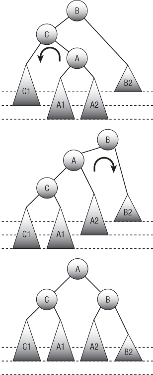
Figure 11.4: A left rotation followed by a right rotation rebalances the tree if the new node is in the left child's right subtree.
You can rebalance the tree in this case with a left rotation followed by a right rotation. The second image in Figure 11.4 shows the tree after a left rotation to change the positions of nodes A and C. At this point, the tree is in the left-left case, like the one shown in Figure 11.1. The left child's subtree is two levels deeper than node B's right subtree. Now you can rebalance the tree the same way you do in the left-left case by using a right rotation. The bottom image in Figure 11.4 shows the resulting balanced tree.
Similar techniques let you rebalance the tree in the right-left case. Use a right rotation to put the tree in the right-right case and then use a left rotation to rebalance the tree.
Deleting Values
You can use the same rotations to rebalance the tree whether you're adding new nodes or removing existing nodes. For example, Figure 11.5 shows the process of removing a node from an AVL tree. The top image shows the original tree. After node 1 is removed, the tree in the middle of the figure is unbalanced at node 3, because that node's left subtree has height 1 and its right subtree has height 3. A left rotation gives the rebalanced tree shown on the bottom.

Figure 11.5: A left rotation rebalances the tree after node 1 is removed.
At all times, an AVL tree containing N nodes has height at most ![]() so it is reasonably short and wide. This means that operations that climb the tree, such as searching for a value, take
so it is reasonably short and wide. This means that operations that climb the tree, such as searching for a value, take ![]() time.
time.
Rebalancing the tree also takes at most ![]() time, so adding or removing a value takes
time, so adding or removing a value takes ![]() time.
time.
2-3 Trees
To keep an AVL tree balanced, you consider the tree's structure at a relatively large scale. The subtrees at any node differ in height by at most 1. If you needed to examine the subtrees to determine their heights, you would need to search the subtrees to their leaf nodes.
To keep a 2-3 tree balanced, you consider its nodes at a smaller scale. Instead of considering entire subtrees at any given node, you consider the number of children each node has.
In a 2-3 tree, every internal node has either two or three children. A node that has two children is called a 2-node, and a node that has three children is called a 3-node. Because every internal node has at least two children, a tree containing N nodes can have a height of at most ![]()
Nodes with two children work the same way that the nodes do in a normal binary tree. Such a node holds a value. When you're searching the tree, you look down the node's left or right branch, depending on whether the target value is less than or greater than the node's value.
Nodes with three children hold two values. When you're searching the tree, you look down this node's left, middle, or right branch, depending on whether the target value is less than the node's first value, between its first and second values, or greater than its second value.
In practice, you can use the same class or structure to represent both kinds of nodes. Just create a node that can hold up to two values and three children. Then add a property that tells how many values are in use. (Note that a leaf node might hold one or two values but has no children.)
Figure 11.6 shows a 2-3 tree. To find the value 76, you would compare 76 to the root node's value 42. The target value 76 is greater than 42, so you move down the branch to the right of the value 42. At the next node, you compare 76 to 69 and 81. The target value 76 is between 69 and 81, so you move down the middle branch. You then find the value 76 in the leaf node.

Figure 11.6: In a 2-3 tree, every internal node has either two or three children.
Searching a 2-3 tree is reasonably simple, but adding and deleting values is a bit harder than it is for a normal binary tree.
Adding Values
To add a new value to the tree, search the tree much as you would search any sorted tree to find the leaf node where the new value belongs. There are two cases, depending on whether the leaf node is full.
First, if the leaf node holds fewer than two values, simply add the new value to the node, keeping it in sorted order with the node's existing value and you're done.
Second, suppose that the leaf node that should hold the new value already holds two values, so it is full. In that case, you split the node into two new nodes, put the smallest value in the left node, put the largest value in the right node, and move the middle value up to the parent node. This is called a node split.
Figure 11.7 shows the process of adding the value 42 to the tree on the left. The value 42 is greater than the value 27 in the root node, so the new value should be placed down the root node's right branch. The node down that branch is a leaf node, so that is where the new value ideally belongs. That node is full, however, so adding the new value would give it three values: 32, 42, and 57. To make room, you split the leaf node into two new nodes holding the smaller and larger values 32 and 57, and you move the middle value up to the parent node. The resulting tree is shown on the right.

Figure 11.7: Adding a new value to a full leaf node forces a node split.
When a node splits, you need to move a value up to its parent node. That may cause the parent node to hold too many values, so it also splits. In the worst case, the series of splits cascades all the way up the tree to the root node, causing a root split. When a root split occurs, the tree grows taller. This is the only way a 2-3 tree grows taller.
In a sorted binary tree, adding values in sorted order is the worst-case scenario and results in a tall, thin tree. If you add N nodes to the tree, the tree has height N.
Figure 11.8 shows a 2-3 tree with the values 1 through 7 added in numeric order. The tree can hold the values 1 and 2 in the root node, so the first image shows the tree already containing those values. Each image shows the next value to be added and the location where it belongs in the tree. If you step through the stages, you'll see that adding the value 4 causes a node split and adding the value 7 causes a root split.

Figure 11.8: Adding a new value to a full leaf node forces a node split
Deleting Values
In theory, deleting a value from a 2-3 tree is about the same as adding one in reverse. Instead of node splits, you may have node merges. In practice, however, the details are fairly complicated.
You can simplify the problem if you can treat all deletions as if they are from a leaf node. If the target value is not in a leaf node, replace it with the rightmost value to the left of it in the tree, just as you would in any sorted tree. The replacement node will be in a leaf node, so now you can treat the situation as if you had removed the rightmost value from that leaf node.
After you remove a value from a node, that node contains either zero values or one value. If it contains one value, you're done.
If the node now contains zero values, you may be able to borrow a value from its sibling node. If the node's sibling has two values, move one into the empty node, and again you're done.
For example, consider the tree shown at the top of Figure 11.9. Suppose you want to remove the value 4 from the root. Start by moving the value 3 into the deleted position to get the tree shown second in the picture.

Figure 11.9: When you delete a value from a node in a 2-3 tree, sometimes a node that is too empty can borrow values from its sibling.
This tree is no longer a 2-3 tree because the internal node A has only one child. In this example, node A's sibling node B has three children, so node A can take one. Move the node containing the value 5 so that it is a child of node A. When you remove that node, you must also remove the value 6 that was used to decide when to move left from node B to the node containing 5. The third tree in Figure 11.9 shows the new situation.
At this point, the value 6 doesn't have a node, and the values in the tree are no longer in sorted order because the value 5 is to the left of value 3. The value 6 is greater than any value in A's subtree, so move it to A's parent. The value that was in that position (3 in this example) is greater than the values in A's original subtree and less than the value borrowed from its sibling (5), so put 3 to the left of the borrowed value.
The bottom tree in Figure 11.9 shows the final result.
One more situation may occur when you delete a value. Suppose that you remove a value from a node. If the node then has only one child and the node's sibling contains only one value, then you can't borrow a node from the sibling. In that case, you can merge the node and its sibling. Not surprisingly, this is called a node merge.
When you merge two nodes, their parent loses a child. If the parent had only two children, it now violates the condition that every internal node in a 2-3 tree must have either two or three children. In that case, you move up the tree and rebalance at that node's parent, either redistributing nodes or merging the parent with its sibling.
For example, consider the tree shown at the top of Figure 11.10 and suppose that you want to delete the value 3. Doing so results in the second tree shown in the figure. This tree is no longer a 2-3 tree because internal node A has only one child.

Figure 11.10: Sometimes when you delete a value from a 2-3 tree, you need to merge two nodes.
Node B also has only two children, so node A cannot borrow a child from it. Instead, you need to merge nodes A and B. Between them, nodes A and B contain two values and have three children, so that works from a space point of view.
When you merge the two nodes, their parent node loses a child, so it must also lose a value. You can move that value into the merged node's subtree.
After you make those rearrangements, the values are no longer in sorted order, so you need to rearrange them a bit. The bottom of Figure 11.10 shows the resulting tree.
In this example, the top node (which ends up holding the value 20) has two children. If it did not, you would have to rebalance the tree at that node's level, either borrowing a child or merging with that node's sibling.
In the worst case, a series of merges can cascade all the way to the tree's root, causing a root merge. This is the only way a 2-3 tree grows shorter.
B-Trees
B-trees (pronounced “bee trees”) are an extension of 2-3 trees. (Or, if you prefer, 2-3 trees are a special case of B-trees.) In a 2-3 tree, every internal node holds one or two values and has two or three branches. In a B-tree of order K, every internal node (except possibly the root) holds between K and ![]() values and has between
values and has between ![]() and
and ![]() branches.
branches.
Because they can hold many values, the internal nodes in a B-tree are often called buckets.
The number of values that a B-tree node can hold is determined by the tree's order. A B-tree of order K has these properties:
- Each node holds at most
 values.
 - Each node, except possibly the root node, holds at least K values.
- An internal node holding M values has
 branches leading to
  children.
 - All leaves are at the same level in the tree.
Because each internal node has at least ![]() branches, the B-tree cannot grow too tall and thin. For example, every internal node in a B-tree of order 9 has at least 10 branches, so a tree holding 1 million values would need to be about
branches, the B-tree cannot grow too tall and thin. For example, every internal node in a B-tree of order 9 has at least 10 branches, so a tree holding 1 million values would need to be about ![]() levels tall. (A complete binary tree would need to be 20 levels tall to hold the same values.)
levels tall. (A complete binary tree would need to be 20 levels tall to hold the same values.)
You search a B-tree much as you search a 2-3 tree. At each node, you find the values between which the target value lies and then move down the corresponding branch.
Figure 11.11 shows a B-tree node of order 2. If you were searching the tree for the value 35, you would move down branch B, because 35 is between the node's values 27 and 36, and branch B is between those values. If you wanted to find the value 50, you would move down branch D, because that is the node's last branch, and the value 50 is greater than all of the node's values.

Figure 11.11: In a B-tree, internal nodes hold several values with branches between them.
Just as searching in a B-tree is similar to searching in a 2-3 tree, adding and removing values in a B-tree is similar to adding and removing values in a 2-3 tree.
Adding Values
To insert a value in a B-tree, locate the leaf node that should contain it. If that node contains fewer than ![]() values, simply add the new value.
values, simply add the new value.
If the node contains ![]() values, there's no room for a new value. If any one of the node's siblings contains fewer than
values, there's no room for a new value. If any one of the node's siblings contains fewer than ![]() values, you can rearrange the values in the siblings so that the new value will fit.
values, you can rearrange the values in the siblings so that the new value will fit.
For example, consider the tree shown at the top of Figure 11.12 and suppose that you want to add the value 17. The leaf that should hold the new value is full. In the tree at the bottom of the figure, the values in the node and its right sibling have been rearranged to make room for the new value. Notice that the dividing value has been changed in the parent node.

Figure 11.12: Sometimes when you add a value to a full B-tree node, you can redistribute values among the node's siblings to make room.
If all of the sibling nodes are full (or if you don't want to rearrange values among siblings, a potentially difficult task), you can split the node into two nodes that each contain 2 × K values. Add the new value to the node's existing values, move the middle value up to be the dividing value in the parent node, and put the remaining values in the two new nodes.
For example, consider the tree shown at the top of Figure 11.13 and suppose that you want to add the value 34. The leaf node and its siblings are all full, so you cannot redistribute values to make room. Instead, you can split the node, as shown at the bottom of the figure.

Figure 11.13: Sometimes when you add a value to a full B-tree node, you must split the node.
When you move a new value up to the parent node, that node may become too full. In that case, you must repeat the process with the parent node, either rearranging values among that node's siblings or splitting that node and moving a value up to its parent.
In the worst case, the split travels all of the way up the tree to the root, where it causes a root split. This is the only way a B-tree grows taller.
Deleting Values
To remove a value from an internal node, swap it with the rightmost value to the left in the tree, as you normally do for sorted trees. Then treat the case as if you were removing the value from a leaf node.
After you remove the value, if the leaf node contains at least K values, you're done. If the leaf node contains fewer than K values, you must rebalance the tree.
If any one of the node's siblings holds more than K values, you can redistribute the values to give the target node K values.
For example, consider the tree shown at the top of Figure 11.14 and suppose that you want to remove the value 32. That would leave its leaf node holding only one value, which is not allowed for a B-tree of degree 2. In the tree at the bottom of the figure, the values in the node and its siblings have been rearranged so that each holds two values.

Figure 11.14: Sometimes when you delete a value from a B-tree node, you can redistribute values among the node's siblings to rebalance the tree.
If none of the node's siblings holds more than K values, you can merge the node with one of its siblings to make a node that holds ![]() values.
values.
For example, consider the tree shown at the top of Figure 11.15 and suppose that you want to delete the value 12. Its leaf node and all of its siblings all hold K values, so you cannot redistribute values. Instead, you can merge the leaf with one of its siblings, as shown at the bottom of the figure.

Figure 11.15: Sometimes when you delete a value from a B-tree node, you must merge the node with a sibling.
When you merge two nodes, the parent node may not hold K values. In that case, you must repeat the process with the parent node, either rearranging values among that node's siblings or merging that node with one of its siblings.
In the worst case, the merge travels all of the way up the tree to the root, where it causes a root merge. This is the only way a B-tree grows shorter.
Balanced Tree Variations
There are many other kinds of balanced tree structures and several variations on the ones that have already been described. The following sections cover two useful modifications that you can make to B-trees. These modifications are described for B-trees, but they also apply to some of the other kinds of balanced trees. In particular, because a 2-3 tree is really just a B-tree of order 1, these techniques apply directly to 2-3 trees.
Top-down B-trees
When you add an item to a B-tree, you first recursively move down into the tree to find the leaf node that should hold it. If that bucket is full, you may need to split it and move an item up to the parent node. As the recursive calls return, they can add a value that has been moved up to the current node and, if that node splits, move another value up the tree. Because these bucket splits occur as the recursive calls return up the tree, this data structure is sometimes called a bottom-up B-tree.
An alternative strategy is to make the algorithm split any full nodes on the way down into the tree. This creates room in the parent node if the algorithm must move a value up the tree. For example, if the leaf node that should hold the new value is full, the algorithm knows that the leaf's parent has room, because if it didn't, it would have been split already. Because these bucket splits occur as the recursion moves down into the tree, this variation is sometimes called a top-down B-tree.
In a top-down B-tree, bucket splits occur sooner than they might otherwise. The top-down algorithm splits a full node even if its children contain lots of unused entries. This means that the tree holds more unused entries than necessary, so it is taller than a bottom-up B-tree would be. However, all that empty space also reduces the chances that adding a new value will cause a long series of bucket splits.
Unfortunately, there is no top-down algorithm for bucket merging. As it moves down into the tree, the algorithm cannot tell if a node will lose a child, so it can't know if it should merge that node with a sibling.
B+trees
B-trees are often used to store large records. For example, a B-tree might hold employee records, each occupying several kilobytes of space. If the records include photographs of the employees, each might hold a few megabytes. The B-tree would organize its data by using some sort of key value, such as employee ID.
In that case, rearranging the items in a bucket would be fairly slow, because the program might need to shuffle many megabytes of data among several nodes. A cascading bucket split could make the algorithm move a huge amount of data.
One way to avoid moving large amounts of data is to place only the key values in the B-tree's internal nodes and then make each node also store a pointer to the rest of the record's data. Now when the algorithm needs to rearrange buckets, it moves only the keys and the record pointers instead of the whole record. This type of tree is called a B+tree (pronounced “bee plus tree”).
Figure 11.16 shows the idea behind B+trees. Here dashed lines indicate links (pointers) from a key to the corresponding data, shown in a box.

Figure 11.16: In a B+tree, values are linked to the corresponding data, shown here in boxes.
B+trees have a couple of advantages in addition to making it faster to rearrange values. First, they let a program easily use multiple trees to manage different keys for the same data. For example, a program might use one B+tree to arrange employee records by employee ID and another B+tree to arrange the same records by Social Security number. Each tree would use the same pointers to refer to the employee records. To find an employee by ID or Social Security number, you would search the appropriate tree and then follow the correct pointer to the actual data.
A second benefit of B+trees is that the nodes could hold more values in the same space. This means that you can increase the tree's degree and make the tree shorter.
For example, suppose that you build an order 2 B-tree so that each node has between three and five children. To hold 1 million records, this tree would need a height between ![]() and
and ![]() . To find an item in this tree, the program might need to search as many as 13 nodes. It is unlikely that all of the tree's records would fit into memory all at once, so this might require 13 disk accesses, which would be relatively slow.
. To find an item in this tree, the program might need to search as many as 13 nodes. It is unlikely that all of the tree's records would fit into memory all at once, so this might require 13 disk accesses, which would be relatively slow.
Now suppose that you store the same 1 million records in a B+tree using nodes that use the same number of kilobytes as the original nodes. Because the B+tree stores only key values in the nodes, its nodes may be able to hold far more keys.
Suppose the new B+tree can store up to 20 employee IDs in the same node space. (The actual value may be much larger, depending on the size of the employee records.) In that case, each node in the tree would have between 11 and 21 children, so the tree could store the same 1 million values with a height between ![]() and
and ![]() . To find an item, the program would need to search only six nodes at most and perform six disk accesses at most, cutting the search time roughly in half.
. To find an item, the program would need to search only six nodes at most and perform six disk accesses at most, cutting the search time roughly in half.
Summary
Like other sorted trees, balanced trees let a program store and find values quickly. By keeping themselves balanced, trees such as AVL trees, 2-3 trees, B-trees, and B+trees ensure that they don't grow too tall and thin, which would ruin their performance.
Adding and removing values in a balanced tree takes longer than it does in an ordinary (nonbalanced) sorted tree. Those operations still take only ![]() time, however, so the theoretical run time is the same even if the actual time is slightly longer. Spending that extra time lets the algorithm guarantee that those operations don't grow to linear time.
time, however, so the theoretical run time is the same even if the actual time is slightly longer. Spending that extra time lets the algorithm guarantee that those operations don't grow to linear time.
Chapter 8 described hash tables, which store and retrieve values even more quickly than balanced trees do. However, hash tables don't allow some of the same features, such as quickly displaying all of the values in the data structure in sorted order.
This chapter and the preceding one describe generic tree algorithms that let you build and traverse trees and balanced trees. The next chapter describes decision trees, which you can use to model and solve a wide variety of problems.
Exercises
You can find the answers to these exercises in Appendix B. Asterisks indicate particularly difficult problems.
- Draw a picture similar to Figure 11.4 showing how to rebalance an AVL tree in the right-left case.
- Draw a series of pictures showing an AVL tree as you add the values 1 through 8 to it in numeric order.
- Rebalance the AVL tree shown in Figure 11.17 after removing node 33.
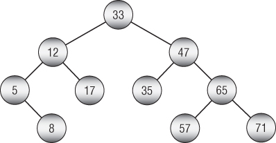
Figure 11.17: Remove value 33 from this AVL tree and rebalance it.
- Draw a series of pictures similar to Figure 11.7 showing how to rebalance the 2-3 tree shown in Figure 11.18 after you add the value 24 to it.

Figure 11.18: Add value 24 to this 2-3 tree and rebalance it.
- Draw a series of pictures similar to Figure 11.9 showing how to remove the value 20 from the 2-3 tree shown in Figure 11.18.
- Draw a series of pictures similar to Figure 11.13 showing how to add the value 56 to the B-tree shown in Figure 11.19.

Figure 11.19: Add value 56 to this B-tree and rebalance it.
- Draw a series of pictures similar to the one shown in Figure 11.14 illustrating how to delete the value 49 from the B-tree you got as the final solution in Exercise 6 above.
- Draw a series of pictures that shows a B-tree of order 2 as you add consecutive numbers 1, 2, 3, and so forth until the root node has four children. How many values does the tree hold at that point?
- Computers usually read data from a hard disk in blocks. Suppose that a computer has a 2 KB block size, and you want to build a B-tree or a B+tree that stores customer records using four blocks per bucket. Assume that each record occupies 1 KB, and you want the key value stored by the tree to be the customer's name, which occupies up to 100 bytes. Also assume that pointers between nodes (or to data in a B+tree) take 8 bytes each. What is the largest order you could use for a B-tree or a B+tree while using four-block buckets? What would be the maximum height of the B-tree and B+tree if they hold 10,000 records?