
4
Multirate Elastic Adaptive Retry Loss Models
In this chapter we consider multirate loss models of random arriving calls not only with elastic bandwidth requirements upon arrival but also elastic bandwidth allocation during service. Calls may retry several times upon arrival, requiring less bandwidth each time, in order to be accepted for service. If call admission is not possible with the last (least) bandwidth requirement then bandwidth compression is attempted.
4.1 The Elastic Single‐Retry Model
4.1.1 The Service System
In the elastic single‐retry model (E‐SRM), we consider a link of capacity ![]() b.u. that accommodates elastic calls of
b.u. that accommodates elastic calls of ![]() service‐classes. Calls of service‐class
service‐classes. Calls of service‐class ![]() follow a Poisson process with mean arrival rate
follow a Poisson process with mean arrival rate ![]() and have a peak‐bandwidth requirement of
and have a peak‐bandwidth requirement of ![]() b.u. and an exponentially distributed service time with mean
b.u. and an exponentially distributed service time with mean ![]() . To introduce bandwidth compression, we permit the occupied link bandwidth
. To introduce bandwidth compression, we permit the occupied link bandwidth ![]() to virtually exceed
to virtually exceed ![]() up to a limit of
up to a limit of ![]() b.u. Let
b.u. Let ![]() be the occupied link bandwidth,
be the occupied link bandwidth, ![]() , when a new service‐class
, when a new service‐class ![]() call arrives in the link. Then, for call admission we consider the following cases:
call arrives in the link. Then, for call admission we consider the following cases:
- (a) If
 , no bandwidth compression takes place and the call is accepted in the link with
  b.u.
b.u. - (b)
If
 , then the call is blocked with
  and retries immediately to be connected in the link with
  . Now if:
- b1)
 , no bandwidth compression occurs and the retry call is accepted in the system with
  and
and  , so that
  ,
, - b2)
 , the retry call is blocked and lost, and
 - b3)
 , the retry call is accepted in the system by compressing its bandwidth requirement
  together with the bandwidth of all in‐service calls of all service‐classes. In that case, the compressed bandwidth of the retry call becomes
  , where
  is the compression factor, common to all service‐classes. Similarly, all in‐service calls, which have been accepted in the link with
  (or
(or  ), compress their bandwidth to
  (or
(or  ) for
) for  . After the compression of all calls, the link state is
  . The minimum value of the compression factor is
  .
.
- b1)
Similar to the E‐EMLM, when a service‐class ![]() call, with bandwidth
call, with bandwidth ![]() (or
(or ![]() ), departs from the system, the remaining in‐service calls of each service‐class
), departs from the system, the remaining in‐service calls of each service‐class ![]() expand their bandwidth in proportion to their initially assigned bandwidth
expand their bandwidth in proportion to their initially assigned bandwidth ![]() (or
(or ![]() ). After bandwidth compression/expansion, elastic service‐class calls increase/decrease their service time so that the product service time by bandwidth remains constant.
). After bandwidth compression/expansion, elastic service‐class calls increase/decrease their service time so that the product service time by bandwidth remains constant.
Similar to the SRM, the steady state probabilities in the E‐SRM do not have a PFS, since LB is destroyed between adjacent states (see Figure 4.1). Thus, the unnormalized values of ![]() can be determined by an approximate but recursive formula, as presented in Section 4.1.2.
can be determined by an approximate but recursive formula, as presented in Section 4.1.2.

Figure 4.1 The state space  and the state transition diagram (Example 4.1).
Table 4.1 The state space ![]() and the occupied link bandwidth (Example 4.1).
and the occupied link bandwidth (Example 4.1).
| (before compr.) | (after compr.) | (before compr.) | (after compr.) | ||||||||
| 0 | 0 | 0 | 1.00 | 0 | 0 | 2 | 0 | 0 | 1.00 | 2 | 2 |
| 0 | 0 | 1 | 1.00 | 2 | 2 | 2 | 0 | 1 | 1.00 | 4 | 4 |
| 0 | 0 | 2 | 1.00 | 4 | 4 | 2 | 0 | 2 | 0.67 | 6 | 4 |
| 0 | 0 | 3 | 0.67 | 6 | 4 | 2 | 1 | 0 | 0.80 | 5 | 4 |
| 0 | 1 | 0 | 1.00 | 3 | 3 | 3 | 0 | 0 | 1.00 | 3 | 3 |
| 0 | 1 | 1 | 0.80 | 5 | 4 | 3 | 0 | 1 | 0.80 | 5 | 4 |
| 1 | 0 | 0 | 1.00 | 1 | 1 | 3 | 1 | 0 | 0.67 | 6 | 4 |
| 1 | 0 | 1 | 1.00 | 3 | 3 | 4 | 0 | 0 | 1.00 | 4 | 4 |
| 1 | 0 | 2 | 0.80 | 5 | 4 | 4 | 0 | 1 | 0.67 | 6 | 4 |
| 1 | 1 | 0 | 1.00 | 4 | 4 | 5 | 0 | 0 | 0.80 | 5 | 4 |
| 1 | 1 | 1 | 0.67 | 6 | 4 | 6 | 0 | 0 | 0.67 | 6 | 4 |
To facilitate the recursive calculation of ![]() , we replace
, we replace ![]() by the state‐dependent compression factors per service‐class
by the state‐dependent compression factors per service‐class ![]() , which have a similar role to
, which have a similar role to ![]() and have already been described in the E‐EMLM. The only difference is that apart from
and have already been described in the E‐EMLM. The only difference is that apart from ![]() , which are given by (3.8), we should also define
, which are given by (3.8), we should also define ![]() to account for retry calls of service‐class
to account for retry calls of service‐class ![]() in state
in state ![]() . The form of
. The form of ![]() is the following [1]:
is the following [1]:

where ![]() ,
, ![]() , and
, and

4.1.2 The Analytical Model
4.1.2.1 Steady State Probabilities
To describe the analytical model in the steady state, we consider a link of capacity ![]() b.u. that accommodates calls of two service‐classes with traffic parameters: (
b.u. that accommodates calls of two service‐classes with traffic parameters: (![]() ) for service‐class 1 and (
) for service‐class 1 and (![]() ) for service‐class 2. Calls of service‐class 2 have retry parameters with
) for service‐class 2. Calls of service‐class 2 have retry parameters with ![]() and
and ![]() . Let
. Let ![]() be the virtual capacity so that the maximum permitted bandwidth compression is
be the virtual capacity so that the maximum permitted bandwidth compression is ![]() for calls of both service‐classes.
for calls of both service‐classes.
Although the E‐SRM is a non‐PFS model, we will use the LB of (3.11), initially for calls of service‐class 1:
where ![]() with
with ![]() , and
, and

Based on (4.4) and multiplying both sides of (4.3) with ![]() , we have:
, we have:
where ![]() and the values of
and the values of ![]() are given by (4.2).
are given by (4.2).
Based on the CAC of the E‐SRM, we consider the following LB equations for calls of service‐class 2:
- (a) No bandwidth compression
(4.6)

where
 with
with  and(4.7)
Based on (4.7) and multiplying both sides of (4.6) with
 , we have:(4.8)
where
 and the values of
  are given by ( 4.2).
 - (b) Bandwidth compression
(4.9)

where
 and(4.10)
Based on (4.10) and multiplying both sides of (4.9) with
 , we have:(4.11)
where
 and the values of
  are given by ( 4.2).
Equations (4.5), (4.8), and (4.11) lead to the following system of equations:
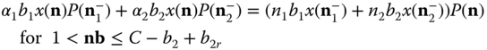


Equations (4.12)–(4.14) can be combined into one equation by assuming that calls with ![]() are negligible when
are negligible when ![]() and calls with
and calls with ![]() are negligible when
are negligible when ![]() :
:

where ![]() for
for ![]() , otherwise
, otherwise ![]() and
and ![]() for
for ![]() , otherwise
, otherwise ![]() .
.
Note that the approximations introduced in (4.15) are similar to those introduced in the STM of [2].
Since ![]() , when
, when ![]() , it is proved in [ 2] (see also (2.9)) that:
, it is proved in [ 2] (see also (2.9)) that:
for ![]() and
and ![]() for
for ![]() , otherwise
, otherwise ![]() .
.
Reminder: To prove (4.16), the migration approximation is needed, which assumes that the population of retry calls of service‐class 2 is negligible in states ![]() .
.
When ![]() and based on ( 4.2), ( 4.15) can be written as:
and based on ( 4.2), ( 4.15) can be written as:
To introduce the link occupancy distribution q(j) in (4.17), we sum both sides of ( 4.17) over the set of states ![]() :
:

Since by definition ![]() , (4.18) is written as:
, (4.18) is written as:
where ![]() for
for ![]() .
.
The combination of ( 4.16) and (4.19) gives the following approximate recursive formula for the calculation of ![]() in the case of two service‐classes, when only calls of service‐class 2 have retry parameters (for
in the case of two service‐classes, when only calls of service‐class 2 have retry parameters (for ![]() ):
):

where ![]() for
for ![]() , otherwise
, otherwise ![]() , and
, and ![]() for
for ![]() , otherwise
, otherwise ![]() .
.
In the case of ![]() service‐classes and assuming that all service‐classes may have retry parameters (4.20) takes the general form:
service‐classes and assuming that all service‐classes may have retry parameters (4.20) takes the general form:

where  ,
,  .
.
4.1.2.2 CBP, Utilization, and Mean Number of In‐service Calls
Having determined the unnormalized values of ![]() , we can calculate [1]:
, we can calculate [1]:
- The CBP of service‐class k calls with
 b.u.,
b.u.,  , via:
(4.22)where
, via:
(4.22)where
 is the normalization constant and
  .
. - The CBP of service‐class
 calls with
  b.u.,
b.u.,  , when
  , via:
(4.23)
, via:
(4.23)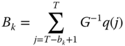
Note that if
 , then
  refers to the
  and the summation in (4.23) should start from
  .
. - The conditional CBP of service‐class
 retry calls given that they have been blocked with their initial bandwidth requirement
  , via:
(4.24)
, via:
(4.24)
- The link utilization,
 , by (3.23).
 - The mean number of service‐class k calls with
 b.u. in state
  , via:
(4.25)
, via:
(4.25)
- The mean number of service‐class
 calls with
  b.u. in state
  , via:
(4.26)where
, via:
(4.26)where
 for
for  , otherwise
  and
and  for
for  , otherwise
  .
. - The mean number of in‐service calls of service‐class
 accepted with
  , via:
(4.27)
, via:
(4.27)
- The mean number of in‐service calls of service‐class
 accepted with
  , via:
(4.28)
, via:
(4.28)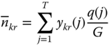
4.2 The Elastic Single‐Retry Model under the BR Policy
4.2.1 The Service System
We now consider the E‐SRM under the BR policy (E‐SRM/BR) with BR parameter ![]() for service‐class
for service‐class ![]() calls (
calls (![]() ). For CAC in the E‐SRM/BR, we consider the following cases:
). For CAC in the E‐SRM/BR, we consider the following cases:
- (a) If
 , no bandwidth compression takes place and the call is accepted in the link with
  b.u.
b.u. - (b)
If
 , then the call is blocked with
  and retries immediately to be connected in the link with
  . Now if:
- b1)
 , no bandwidth compression occurs and the retry call is accepted in the system with
  and
and  , so that
  ,
, - b2)
 , the retry call is blocked and lost, and
 - b3)
 , the retry call is accepted in the system by compressing its bandwidth requirement
  together with the bandwidth of all in‐service calls of all service‐classes. In that case, the compressed bandwidth of the retry call becomes
  where
where  is the compression factor, common to all service‐classes. Similarly, all in‐service calls, which have been accepted in the link with
  (or
(or  ), compress their bandwidth to
  (or
(or  ) for
) for  . After the compression of all calls the link state is
  . The minimum value of the compression factor is
  .
.
- b1)
As far as the values of ![]() ,
, ![]() , and
, and ![]() are concerned they are determined by (3.8), (4.1), and ( 4.2), respectively.
are concerned they are determined by (3.8), (4.1), and ( 4.2), respectively.
4.2.2 The Analytical Model
4.2.2.1 Link Occupancy Distribution
In the E‐SRM/BR, the recursive calculation of ![]() is based on the Roberts method (see Section 1.3.2.2), which leads to the formula [4]:
is based on the Roberts method (see Section 1.3.2.2), which leads to the formula [4]:

where  and
and  .
.
4.2.2.2 CBP, Utilization, and Mean Number of In‐service Calls
Based on (4.29), the following performance measures can be calculated:
- The CBP of service‐class
 calls with
  b.u.,
b.u.,  , via:
(4.30)where
, via:
(4.30)where
 is the normalization constant and
  .
. - The CBP of service‐class
 calls with
  b.u.,
b.u.,  , when
  , via:
(4.31)
, via:
(4.31)
Note that if
 , then
  refers to the
  and the summation in (4.31) should start from
  .
. - The conditional CBP of service‐class
 retry calls given that they have been blocked with their initial bandwidth requirement
  , via:
(4.32)
, via:
(4.32)
- The link utilization,
 , via (3.23).
 - The mean number of service‐class
 calls with
  b.u. in state
  , via (4.25), and the mean number of service‐class
  calls with
  b.u. in state
  ,
,  , via (4.26).
 - The mean number of in‐service calls of service‐class
 accepted in the system with
  , via (4.27), and the mean number of in‐service calls of service‐class
  accepted in the system with
  , via (4.28).
4.3 The Elastic Multi‐Retry Model
4.3.1 The Service System
Similar to the MRM, in the elastic multi‐retry model (E‐MRM) a blocked call of service‐class ![]() can have more than one retry parameter
can have more than one retry parameter ![]() for
for ![]() , where
, where ![]() and
and ![]() .
.
To simply describe the CAC, we assume that a service‐class ![]() call has a peak‐bandwidth requirement of
call has a peak‐bandwidth requirement of ![]() b.u. and may retry twice to be connected in the system, the first time with
b.u. and may retry twice to be connected in the system, the first time with ![]() and the second time (if blocked with
and the second time (if blocked with ![]() ) with
) with ![]() . Then, for call admission, we consider the following cases:
. Then, for call admission, we consider the following cases:
- (a) If
 , no bandwidth compression takes place and the call is accepted in the link with
  b.u.
b.u. - (b) If
 , then the call is blocked with
  and retries immediately to be connected in the link with
  . If
. If  , the retry call is accepted in the system with
  and
and  (no bandwidth compression occurs).
 - (c)
If
 , the retry call is blocked with
  and immediately retries with
  . Now if:
- c1)
 , the retry call is accepted in the system with
  and
and  (no bandwidth compression occurs).
 - c2)
 , the retry call is blocked and lost, and
 - c3)
 , the retry call is accepted in the system by compressing its bandwidth requirement
  together with the bandwidth of all in‐service calls of all service‐classes. In that case, the compressed bandwidth of the retry call becomes
  , where
  is the compression factor, common to all service‐classes. Similarly, all in‐service calls, which have been accepted in the link with
  (or
(or  or
or  ), compress their bandwidth to
  (or
(or  or
or  ) for
) for  . After the compression of all calls the link state is
  . The minimum value of the compression factor is
  .
.
- c1)
Similar to the E‐SRM, when a service‐class ![]() call, with bandwidth
call, with bandwidth ![]() (or
(or ![]() or
or ![]() ), departs from the system, the remaining in‐service calls of each service‐class
), departs from the system, the remaining in‐service calls of each service‐class ![]() expand their bandwidth in proportion to their initially assigned bandwidth
expand their bandwidth in proportion to their initially assigned bandwidth ![]() (or
(or ![]() or
or ![]() ). After bandwidth compression/expansion, elastic service‐class calls increase/decrease their service time so that the product service time by bandwidth remains constant.
). After bandwidth compression/expansion, elastic service‐class calls increase/decrease their service time so that the product service time by bandwidth remains constant.
Similar to the E‐SRM, the steady state probabilities in the E‐MRM do not have a PFS. Thus, the unnormalized values of ![]() can be determined by an approximate but recursive formula, as presented in Section 4.3.2.
can be determined by an approximate but recursive formula, as presented in Section 4.3.2.
To facilitate the recursive calculation of ![]() , we replace
, we replace ![]() by the state‐dependent compression factors per service‐class
by the state‐dependent compression factors per service‐class ![]() ,
, ![]() , and
, and ![]() ,
, ![]() . The values of
. The values of ![]() are given by (3.8), while those of
are given by (3.8), while those of ![]() are determined by:
are determined by:

where  ,
,  ,
,  , and
, and

4.3.2 The Analytical Model
4.3.2.1 Steady State Probabilities
Following the analysis of Section 4.1.2.1, the calculation of the unnormalized values of ![]() is based on an approximate but recursive formula whose proof is similar to that of ( 4.21) [ 1]:
is based on an approximate but recursive formula whose proof is similar to that of ( 4.21) [ 1]:

where ![]() ,
,  and
and  .
.
4.3.2.2 CBP, Utilization, and Mean Number of In‐service Calls
Having determined the unnormalized values of ![]() via (4.35) we can calculate [ 1]:
via (4.35) we can calculate [ 1]:
- The final CBP of service‐class
 calls with their last bandwidth requirement
  b.u.,
b.u.,  , via:
(4.36)where
, via:
(4.36)where
 is the normalization constant.
 - The CBP of service‐class k calls with
 b.u.,
b.u.,  , via ( 4.23).
 - The conditional CBP of service‐class
 retry calls with
  given that they have been blocked with their initial bandwidth requirement
  , via:
(4.37)
, via:
(4.37)
- The link utilization,
 , by (3.23).
 - The mean number of service‐class
 calls with
  b.u. in state
  , via ( 4.25).
 - The mean number of service‐class
 calls with
  b.u. in state
  , via:
(4.38)
, via:
(4.38)
- The mean number of in‐service calls of service‐class
 accepted with
  , via ( 4.27).
 - The mean number of in‐service calls of service‐class
 accepted with
  , via:
(4.39)
, via:
(4.39)
4.4 The Elastic Multi‐Retry Model under the BR Policy
4.4.1 The Service System
Compared to the E‐SRM/BR, in the elastic multi‐retry model under the BR policy (E‐MRM/BR) with BR parameter ![]() for service‐class
for service‐class ![]() calls (
calls (![]() ), blocked calls of service‐class
), blocked calls of service‐class ![]() can retry more than once to be connected in the system.
can retry more than once to be connected in the system.
To facilitate the recursive calculation of ![]() in the E‐MRM/BR, we replace
in the E‐MRM/BR, we replace ![]() by the state‐dependent compression factors per service‐class
by the state‐dependent compression factors per service‐class ![]() , and
, and ![]() ,
, ![]() . The values of
. The values of ![]() and
and ![]() are given by (3.8) and (4.33), respectively.
are given by (3.8) and (4.33), respectively.
4.4.2 The Analytical Model
4.4.2.1 Steady State Probabilities
Following the analysis of Section 4.2.2.1, the calculation of the unnormalized values of ![]() is based on an approximate but recursive formula whose proof is similar to that of ( 4.29) [ 4]:
is based on an approximate but recursive formula whose proof is similar to that of ( 4.29) [ 4]:

where  ,
,  ,
,  ,
, 
4.4.2.2 CBP, Utilization, and Mean Number of In‐service Calls
Having determined the unnormalized values of ![]() via (4.40) we can calculate:
via (4.40) we can calculate:
- The final CBP of service‐class
 calls with their last bandwidth requirement
  b.u.,
b.u.,  , via:
(4.41)where
, via:
(4.41)where
 is the normalization constant.
 - The CBP of service‐class
 calls with
  b.u.,
b.u.,  , via ( 4.31).
 - The conditional CBP of service‐class
 retry calls with
  given that they have been blocked with their initial bandwidth requirement
  , via:
(4.42)
, via:
(4.42)
- The link utilization,
 , by (3.23).
 - The mean number of service‐class
 calls with
  b.u. in state
  , via ( 4.25).
 - The mean number of service‐class
 calls with
  b.u. in state
  , via (4.38).
 - The mean number of in‐service calls of service‐class
 accepted with
  , via ( 4.27).
 - The mean number of in‐service calls of service‐class
 accepted with
  , via (4.39).
4.5 The Elastic Adaptive Single‐Retry Model
4.5.1 The Service System
In the elastic adaptive single‐retry model (EA‐SRM), we consider a link of capacity ![]() b.u. that accommodates
b.u. that accommodates ![]() service‐classes which are distinguished into
service‐classes which are distinguished into ![]() elastic service‐classes and
elastic service‐classes and ![]() adaptive service‐classes. Calls of service‐class
adaptive service‐classes. Calls of service‐class ![]() follow a Poisson process with an arrival rate
follow a Poisson process with an arrival rate ![]() and have a peak‐bandwidth requirement of
and have a peak‐bandwidth requirement of ![]() b.u. and an exponentially distributed service time with mean
b.u. and an exponentially distributed service time with mean ![]() . The bandwidth compression/expansion mechanism and the CAC of the EA‐SRM are the same as those of the E‐SRM (Section 4.1.1). The only difference is that adaptive calls do not alter their service time after bandwidth compression/expansion.
. The bandwidth compression/expansion mechanism and the CAC of the EA‐SRM are the same as those of the E‐SRM (Section 4.1.1). The only difference is that adaptive calls do not alter their service time after bandwidth compression/expansion.
Similar to the E‐SRM, the steady state probabilities in the EA‐SRM do not have a PFS, since LB is destroyed between adjacent states (see Figure 4.9). Thus, the unnormalized values of ![]() can be determined by an approximate but recursive formula, as presented in Section 4.5.2.
can be determined by an approximate but recursive formula, as presented in Section 4.5.2.

Figure 4.9 The state space  and the state transition diagram (Example 4.13).
To facilitate the recursive calculation of ![]() , we replace
, we replace ![]() by the state‐dependent compression factors per service‐class
by the state‐dependent compression factors per service‐class ![]() and
and ![]() which have already been described in the E‐SRM. The only difference compared to the E‐SRM has to do with the determination of
which have already been described in the E‐SRM. The only difference compared to the E‐SRM has to do with the determination of ![]() which is now given by [5]:
which is now given by [5]:

where ![]() and
and ![]() .
.
4.5.2 The Analytical Model
4.5.2.1 Steady State Probabilities
To describe the analytical model in the steady state, we consider a link of capacity ![]() b.u. that accommodates calls of two service‐classes with traffic parameters: (
b.u. that accommodates calls of two service‐classes with traffic parameters: (![]() ) for service‐class 1 and (
) for service‐class 1 and (![]() ) for service‐class 2. Service‐class 1 is adaptive while service‐class 2 is elastic. Only calls of service‐class 2 have retry parameters with
) for service‐class 2. Service‐class 1 is adaptive while service‐class 2 is elastic. Only calls of service‐class 2 have retry parameters with ![]() and
and ![]() . Let
. Let ![]() be the limit up to which bandwidth compression is permitted for calls of both service‐classes.
be the limit up to which bandwidth compression is permitted for calls of both service‐classes.
Although the EA‐SRM is a non‐PFS model we will use the LB of ( 4.3), initially for calls of service‐class 1. As far as ![]() is concerned it is determined by ( 4.4). Based on ( 4.4) and multiplying both sides of ( 4.3) with
is concerned it is determined by ( 4.4). Based on ( 4.4) and multiplying both sides of ( 4.3) with ![]() and
and ![]() , we have:
, we have:
where ![]() and the values of
and the values of ![]() are given by ( 4.43).
are given by ( 4.43).
Based on the CAC of the EA‐SRM, we consider the following LB equations for calls of service‐class 2:
- No bandwidth compression: in this case, we use ( 4.8) of the E‐SRM.
- Bandwidth compression: in this case, we use ( 4.11) of the E‐SRM.
Equations (4.44), ( 4.8) and ( 4.11) lead to the following system of equations:


Equations (4.45)–(4.47) can be combined into one equation by assuming that calls with ![]() are negligible when
are negligible when ![]() and calls with
and calls with ![]() are negligible when
are negligible when ![]() :
:

where ![]() for
for ![]() , otherwise
, otherwise ![]() and
and ![]() for
for ![]() , otherwise
, otherwise ![]() .
.
At this point, we derive a formula for ![]() (which is a simplified version of ( 4.43)) by making the following assumptions:
(which is a simplified version of ( 4.43)) by making the following assumptions:
- When
 , the bandwidth of all in‐service calls should be compressed by
  , so that:
(4.49)
, so that:
(4.49)
- We keep the product service time by bandwidth of service‐class
 calls (elastic or adaptive) in state
  of the initial Markov chain (with
  ) equal to the corresponding product in the same state
  of the modified Markov chain (with
  and
and  ):
(4.50)
):
(4.50)
By substituting (4.50) in (4.49) we obtain:
where ![]() and
and ![]() are given by (3.8), and
are given by (3.8), and ![]() by ( 4.1).
by ( 4.1).
Equation (4.51), due to (3.8) and ( 4.1), is written as:

Based on (4.52), we consider again (4.48). Since ![]() , when
, when ![]() , we have ( 4.16).
, we have ( 4.16).
When ![]() and based on ( 4.52), ( 4.48) can be written as:
and based on ( 4.52), ( 4.48) can be written as:
since ![]() , when
, when ![]() .
.
To introduce the link occupancy distribution ![]() in (4.53), we sum both sides of ( 4.53) over the set of states
in (4.53), we sum both sides of ( 4.53) over the set of states ![]() :
:

Since by definition ![]() , (4.54) is written as:
, (4.54) is written as:
where ![]() for
for ![]() .
.
The combination of ( 4.16) and (4.55) gives the following approximate recursive formula for the calculation of ![]() in the case of two service‐classes when service‐class 1 is adaptive, service‐class 2 is elastic, and only calls of service‐class 2 have retry parameters:
in the case of two service‐classes when service‐class 1 is adaptive, service‐class 2 is elastic, and only calls of service‐class 2 have retry parameters:

where ![]() , and
, and ![]() for
for ![]() , otherwise
, otherwise ![]() , while
, while ![]() for
for ![]() , otherwise
, otherwise ![]() .
.
In the case of ![]() service‐classes and assuming that all service‐classes may have retry parameters, (4.56) takes the general form [ 5]:
service‐classes and assuming that all service‐classes may have retry parameters, (4.56) takes the general form [ 5]:

where  .
.
4.5.2.2 CBP, Utilization, and Mean Number of In‐service Calls
Having determined the unnormalized values of ![]() , we can calculate:
, we can calculate:
- The CBP of service‐class
 calls with
  b.u.,
b.u.,  , via (4.22).
 - The CBP of service‐class
 calls with
  b.u.,
b.u.,  , via ( 4.23).
 - The conditional CBP of service‐class
 retry calls given that they have been blocked with their initial bandwidth requirement
  , via (4.24).
 - The link utilization,
 , via (3.23).
 - The mean number of elastic service‐class
 calls with
  b.u. in state
  , via ( 4.25).
 - The mean number of elastic service‐class
 calls with
  b.u. in state
  , via ( 4.26).
 - The mean number of adaptive service‐class
 calls with
  b.u. in state
  , via:
(4.58)
, via:
(4.58)
- The mean number of adaptive service‐class
 calls with
  b.u. in state
  , via:
(4.59)
, via:
(4.59)
- The mean number of in‐service calls of service‐class
 accepted with
  , via ( 4.27).
 - The mean number of in‐service calls of service‐class
 accepted with
  , via ( 4.28).
4.6 The Elastic Adaptive Single‐Retry Model under the BR Policy
4.6.1 The Service System
We now consider the EA‐SRM under the BR policy (EA‐SRM/BR) with BR parameter ![]() for service‐class
for service‐class ![]() calls (
calls (![]() ). The CAC in the EA‐SRM/BR is the same as that of the E‐SRM/BR. As far as the values of
). The CAC in the EA‐SRM/BR is the same as that of the E‐SRM/BR. As far as the values of ![]() ,
, ![]() , and
, and ![]() are concerned they are determined by (3.8), ( 4.1), and ( 4.43), respectively.
are concerned they are determined by (3.8), ( 4.1), and ( 4.43), respectively.
4.6.2 The Analytical Model
4.6.2.1 Link Occupancy Distribution
In the EA‐SRM/BR, the recursive calculation of ![]() is based on the Roberts method (see Section 1.3.2.2), which leads to the formula [ 4]:
is based on the Roberts method (see Section 1.3.2.2), which leads to the formula [ 4]:

where  .
.
4.6.2.2 CBP, Utilization, and Mean Number of In‐service Calls
Based on (4.60), the following performance measures can be calculated:
- The CBP of service‐class
 calls with
  b.u.,
b.u.,  , via (4.30).
 - The CBP of service‐class
 calls with
  b.u.,
b.u.,  , via ( 4.31).
 - The conditional CBP of service‐class
 retry calls given that they have been blocked with their initial bandwidth requirement
  via (4.32).
 - The link utilization,
 , via (3.23).
 - The mean number of service‐class
 calls with
  b.u. in state
  , via (4.58), and the mean number of service‐class
  calls with
  b.u. in state
  , via (4.59).
 - The mean number of in‐service calls of service‐class
 accepted in the system with
  , via ( 4.27), and the mean number of in‐service calls of service‐class
  accepted in the system with
  , via ( 4.28).
4.7 The Elastic Adaptive Multi‐Retry Model
4.7.1 The Service System
Similar to the E‐MRM, in the elastic adaptive multi‐retry model (EA‐MRM) a blocked call of service‐class ![]() can have more than one retry parameter
can have more than one retry parameter ![]() for
for ![]() , where
, where ![]() and
and ![]() . The call admission in the EA‐MRM is the same as the E‐MRM with the exception that adaptive calls do not alter their service time when their bandwidth is compressed/expanded.
. The call admission in the EA‐MRM is the same as the E‐MRM with the exception that adaptive calls do not alter their service time when their bandwidth is compressed/expanded.
Similar to the EA‐SRM, the steady state probabilities in the EA‐MRM do not have a PFS. Thus, the unnormalized values of ![]() can be determined by an approximate but recursive formula, as presented in Section 4.7.2.
can be determined by an approximate but recursive formula, as presented in Section 4.7.2.
To facilitate the recursive calculation of ![]() , we replace
, we replace ![]() by the state‐dependent compression factors per service‐class
by the state‐dependent compression factors per service‐class ![]() and
and ![]() ,
, ![]() whose values are given by (3.8) and ( 4.33), respectively. Due to the existence of adaptive traffic, the values of
whose values are given by (3.8) and ( 4.33), respectively. Due to the existence of adaptive traffic, the values of ![]() are given by the following formula:
are given by the following formula:

where  ,
,  and
and ![]() .
.
4.7.2 The Analytical Model
4.7.2.1 Steady State Probabilities
Following the analysis of Section 4.5.2.1, the calculation of the unnormalized values of ![]() is based on an approximate but recursive formula whose proof is similar to that of ( 4.57) [ 5]:
is based on an approximate but recursive formula whose proof is similar to that of ( 4.57) [ 5]:

where 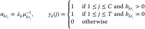 , and
, and  .
.
4.7.2.2 CBP, Utilization, and Mean Number of In‐service Calls
Having determined the unnormalized values of ![]() via (4.62) we can calculate [ 5]:
via (4.62) we can calculate [ 5]:
- The final CBP of service‐class k calls with their last bandwidth requirement
 b.u.,
b.u.,  , via (4.36).
 - The CBP of service‐class
 calls with
  b.u.,
b.u.,  , via ( 4.23).
 - The conditional CBP of service‐class
 retry calls with
  given that they have been blocked with their initial bandwidth requirement
  , via (4.37).
 - The link utilization,
 , by (3.23).
 - The mean number of elastic service‐class
 calls with
  b.u. in state
  , via ( 4.25).
 - The mean number of elastic service‐class
 calls with
  b.u. in state
  , via ( 4.38).
 - The mean number of adaptive service‐class
 calls with
  b.u. in state
  , via ( 4.58).
 - The mean number of adaptive service‐class
 calls with
  b.u. in state
  :
(4.63)
:
(4.63)
- The mean number of in‐service calls of service‐class
 accepted with
  , via ( 4.27).
 - The mean number of in‐service calls of service‐class
 accepted with
  , via ( 4.39).
4.8 The Elastic Adaptive Multi‐Retry Model under the BR Policy
4.8.1 The Service System
Compared to the EA‐SRM/BR, in the elastic adaptive multi‐retry model under the BR policy (EA‐MRM/BR) with BR parameter ![]() for service‐class
for service‐class ![]() calls (
calls (![]() ), blocked calls of service‐class
), blocked calls of service‐class ![]() can retry more than once to be connected in the system.
can retry more than once to be connected in the system.
To facilitate the recursive calculation of ![]() in the EA‐MRM/BR, we replace
in the EA‐MRM/BR, we replace ![]() by the state‐dependent compression factors per service‐class
by the state‐dependent compression factors per service‐class ![]() and
and ![]() ,
, ![]() . The values of
. The values of ![]() and
and ![]() are given by (3.8) and ( 4.33), respectively.
are given by (3.8) and ( 4.33), respectively.
4.8.2 The Analytical Model
4.8.2.1 Steady State Probabilities
Following the analysis of Section 4.6.2.1, the calculation of the unnormalized values of ![]() is based on an approximate but recursive formula whose proof is similar to that of ( 4.60) [3]:
is based on an approximate but recursive formula whose proof is similar to that of ( 4.60) [3]:

where 

4.8.2.2 CBP, Utilization, and Mean Number of In‐service Calls
Having determined the unnormalized values of ![]() via (4.64) we can calculate:
via (4.64) we can calculate:
- The final CBP of service‐class
 calls with their last bandwidth requirement
  b.u.,
b.u.,  , via (4.41).
 - The CBP of service‐class k calls with
 b.u.,
b.u.,  , via ( 4.31).
 - The conditional CBP of service‐class
 retry calls with
  given that they have been blocked with their initial bandwidth requirement
  , via (4.42).
 - The link utilization,
 , by (3.23).
 - The mean number of elastic service‐class
 calls with
  b.u. in state
  , via ( 4.25).
 - The mean number of elastic service‐class
 calls with
  b.u. in state
  , via ( 4.38).
 - The mean number of adaptive service‐class
 calls with
  b.u. in state
  , via ( 4.58).
 - The mean number of adaptive service‐class
 calls with
  b.u. in state
  , via (4.63).
 - The mean number of in‐service calls of service‐class
 accepted in the system with
  , via ( 4.27).
 - The mean number of in‐service calls of service‐class
 accepted in the system with
  , via ( 4.39).
4.9 Applications
Since the multirate elastic adaptive retry loss models are a combination of the retry loss models (see Chapter 2) and the elastic adaptive loss models (see Chapter ), the interested reader may refer to Sections 2.11 and 3.7 for possible applications.
4.10 Further Reading
Similar to the previous section, the interested reader may refer to the corresponding sections of Chapter 2(Section 2.12) and Chapter 3(Section 3.8). In addition to these sections, interesting extensions of the models presented in this chapter have been proposed in [6]. More precisely, in [ 6] the case of finite sources is considered as well as the application of the BR and TH policies.
References
- 1 I. Moscholios, V. Vassilakis, J. Vardakas and M. Logothetis, Retry loss models supporting elastic traffic. Advances in Electronics and Telecommunications, Poznan University of Technology, Poland, 2,(3):8–13, September 2011.
- 2 J. Kaufman, Blocking with retrials in a completely shared resource environment. Performance Evaluation, 15(2):99–113, June 1992.
- 3 I. Moscholios, V. Vassilakis, M. Logothetis and J. Vardakas, Erlang–Engset multirate retry loss models for elastic and adaptive traffic under the bandwidth reservation policy. International Journal on Advances in Networks and Services, 7(1&2):12–24, July 2014.
- 4 I. Moscholios, V. Vassilakis, M. Logothetis and M. Koukias, QoS equalization in a multirate loss model of elastic and adaptive traffic with retrials. 5th International Conference on Emerging Network Intelligence, EMERGING, Porto, Portugal, October 2013.
- 5 I. Moscholios, V. Vassilakis, J. Vardakas and M. Logothetis, Call blocking probabilities of elastic and adaptive traffic with retrials. Proceedings of the 8th Advanced International Conference on Telecommunications, AICT, Stuttgart, Germany, 27 May–1 June 2012.
- 6 I. Moscholios, M. Logothetis, J. Vardakas and A. Boucouvalas, Congestion probabilities of elastic and adaptive calls in Erlang–Engset multirate loss models under the threshold and bandwidth reservation policies. Computer Networks, 92(Part 1):1–23, December 2015.