7
Finite Multirate Retry Threshold Loss Models
We consider multirate loss models of quasi‐random arriving calls with elastic bandwidth requirements and fixed bandwidth allocation during service. Calls may retry several times upon arrival (requiring less bandwidth each time) in order to be accepted for service. Alternatively, new calls may request less bandwidth according to the occupied link bandwidth indicated by threshold(s).
7.1 The Finite Single‐Retry Model
7.1.1 The Service System
In the finite single‐retry model (f‐SRM), a single link of capacity ![]() b.u. accommodates calls of
b.u. accommodates calls of ![]() service‐classes under the CS policy. Calls of service class
service‐classes under the CS policy. Calls of service class ![]() come from a finite source population
come from a finite source population ![]() . The mean arrival rate of service‐class
. The mean arrival rate of service‐class ![]() idle sources is given by
idle sources is given by ![]() , where
, where ![]() is the number of in‐service calls and
is the number of in‐service calls and ![]() is the arrival rate per idle source. The offered traffic‐load per idle source of service‐class
is the arrival rate per idle source. The offered traffic‐load per idle source of service‐class ![]() is given by
is given by ![]() (in erl). Note that if
(in erl). Note that if ![]() for
for ![]() , and the total offered traffic‐load remains constant, then the call arrival process is Poisson. A new call of service‐class
, and the total offered traffic‐load remains constant, then the call arrival process is Poisson. A new call of service‐class ![]() has a peak‐bandwidth requirement of
has a peak‐bandwidth requirement of ![]() b.u. and an exponentially distributed service time with mean
b.u. and an exponentially distributed service time with mean ![]() . If the initially required b.u. are not available in the link, the call is blocked and immediately retries to be connected in the system with
. If the initially required b.u. are not available in the link, the call is blocked and immediately retries to be connected in the system with ![]() b.u. while the mean of the new service time increases to
b.u. while the mean of the new service time increases to ![]() so that the product bandwidth requirement by service time remains constant [1]. If the
so that the product bandwidth requirement by service time remains constant [1]. If the ![]() b.u. are not available the call is blocked and lost. The CAC mechanism of a call of service‐class
b.u. are not available the call is blocked and lost. The CAC mechanism of a call of service‐class ![]() is identical to that of Figure 2.2 of the SRM, i.e., a new call of service‐class
is identical to that of Figure 2.2 of the SRM, i.e., a new call of service‐class ![]() is blocked with
is blocked with ![]() b.u. if
b.u. if ![]() and is accepted with
and is accepted with ![]() if
if ![]() , where
, where ![]() and
and ![]() are the in‐service calls of service‐class
are the in‐service calls of service‐class ![]() accepted with
accepted with ![]() b.u., respectively.
b.u., respectively.
The comparison of the f‐SRM with the EnMLM reveals similar differences to those described in Section 2.1.1 for the SRM and the EMLM.
7.1.2 The Analytical Model
7.1.2.1 Steady State Probabilities
To describe the analytical model in the steady state, let us concentrate on a single link of capacity C b.u. that accommodates only two service‐classes with the following traffic characteristics: ![]() . Blocked calls of service‐class 2 may retry with parameters
. Blocked calls of service‐class 2 may retry with parameters ![]() while blocked calls of service‐class 1 do not retry. Although the f‐SRM does not have a PFS, we assume that the LB equation (6.33), proposed in the EnMLM, does hold, that is [ 1]:
while blocked calls of service‐class 1 do not retry. Although the f‐SRM does not have a PFS, we assume that the LB equation (6.33), proposed in the EnMLM, does hold, that is [ 1]:
or, due to the fact that ![]() in the equivalent stochastic system:
in the equivalent stochastic system:
This assumption is important for the derivation of an approximate but recursive formula for the ![]() . If
. If ![]() , when a new call of service‐class 2 arrives in the system this call is blocked and retries to be connected with
, when a new call of service‐class 2 arrives in the system this call is blocked and retries to be connected with ![]() b.u. If
b.u. If ![]() , the retry call will be accepted in the system. To describe this situation we need an additional LB equation [ 1]:
, the retry call will be accepted in the system. To describe this situation we need an additional LB equation [ 1]:
where ![]() is the offered traffic‐load per idle source of service‐class 2 with
is the offered traffic‐load per idle source of service‐class 2 with ![]() , and
, and ![]() is the mean number of service‐class 2 calls accepted in state
is the mean number of service‐class 2 calls accepted in state ![]() with
with ![]() .
.
Multiplying (7.3) with ![]() , we have for
, we have for ![]() :
:
Multiplying both sides of (7.2) with ![]() , we have for
, we have for ![]() :
:

Adding (7.4) to (7.5), and since ![]() , we obtain:
, we obtain:

Apart from the assumption of the LB equation ( 7.3), another approximation is necessary for the recursive calculation of ![]() :
:
In (7.7), the value of ![]() is considered negligible compared to
is considered negligible compared to ![]() when
when ![]() . This is the migration approximation (see Section 2.1.2.1). Due to ( 7.7), equation ( 7.5) is written as (for
. This is the migration approximation (see Section 2.1.2.1). Due to ( 7.7), equation ( 7.5) is written as (for ![]() :
:
The combination of (7.6) and (7.8) gives an approximate formula for the determination of ![]() in the f‐SRM, assuming that only calls of service‐class 2 can retry [ 1]:
in the f‐SRM, assuming that only calls of service‐class 2 can retry [ 1]:

where ![]() , and
, and ![]() when
when ![]() (otherwise
(otherwise ![]() ).
).
The generalization of (7.9) in the case of ![]() service‐classes, where all service‐classes may retry, is as follows [ 1]:
service‐classes, where all service‐classes may retry, is as follows [ 1]:

where ![]() when
when ![]() (otherwise
(otherwise ![]() ).
).
Note that if ![]() , for
, for ![]() , and the total offered traffic‐load remains constant, then we have the recursion (2.10) of the SRM.
, and the total offered traffic‐load remains constant, then we have the recursion (2.10) of the SRM.
7.1.2.2 TC Probabilities, CBP, Utilization, and Mean Number of In‐service Calls
The following performance measures can be determined based on (7.10):
- The TC probabilities of service‐class k calls with
 b.u.,
b.u.,  , via (6.35).
 - The TC probabilities of service‐class k calls with
 b.u.,
b.u.,  , via:
(7.11)where
, via:
(7.11)where
 is the normalization constant.
 - The CBP (or CC probabilities) of service‐class k calls with
 (without retrial),
  , via (6.35) but for a system with
  traffic sources.
 - The CBP (or CC probabilities) of service‐class k calls with
 ,
,  , via (7.11) but for a system with
  traffic sources.
 - The conditional TC probabilities of service‐class k retry calls given that they have been blocked with their initial bandwidth requirement
 , via:
(7.12)
, via:
(7.12)
- The link utilization,
 , via (6.36).
 - The average number of service‐class k calls in the system accepted with
 b.u.,
b.u.,  , via (6.37), while the mean number of service‐class k calls with
  given that the system state is
  , via (6.38).
 - The average number of service‐class k calls in the system accepted with
 ,
,  , via:
(7.13)where
, via:
(7.13)where
 is the average number of service‐class k calls with
  given that the system state is
  , and is determined by:
(7.14)where
, and is determined by:
(7.14)where
 and
and  when
when  .
.
The determination of ![]() via ( 7.10), and consequently of all performance measures, requires the values of
via ( 7.10), and consequently of all performance measures, requires the values of ![]() and
and ![]() , which are unknown. In [ 1–3] give a method for the determination of
, which are unknown. In [ 1–3] give a method for the determination of ![]() and
and ![]() in each state
in each state ![]() via an equivalent stochastic system, with the same traffic parameters and the same set of states, as already described for the proof of (6.27) in the EnMLM. However, the state space determination of the equivalent system is complex, even for small capacity systems that serve many service‐classes with the ability to retry.
via an equivalent stochastic system, with the same traffic parameters and the same set of states, as already described for the proof of (6.27) in the EnMLM. However, the state space determination of the equivalent system is complex, even for small capacity systems that serve many service‐classes with the ability to retry.
As already mentioned, the determination of an equivalent system is complex, especially when calls retry many times. To circumvent this problem we present, in the next section, the algorithm of Section 6.2.2.3 (initially proposed for the EnMLM) for the f‐SRM.
7.1.2.3 An Approximate Algorithm for the Determination of  in the f‐SRM
Contrary to ( 7.10), which requires enumeration and processing of the state space, the algorithm presented herein is much simpler and easy to implement [4,5].

7.2 The Finite Single‐Retry Model under the BR Policy
7.2.1 The Service System
In the f‐SRM under the BR policy (f‐SRM/BR), ![]() b.u. are reserved to benefit calls of all other service‐classes apart from service‐class k. The application of the BR policy in the f‐SRM is similar to that of the SRM/BR as the following example shows.
b.u. are reserved to benefit calls of all other service‐classes apart from service‐class k. The application of the BR policy in the f‐SRM is similar to that of the SRM/BR as the following example shows.
7.2.2 The Analytical Model
7.2.2.1 Link Occupancy Distribution
In the f‐SRM/BR, the unnormalized values of ![]() can be calculated in an approximate way according to the Roberts method (see Section 1.3.2.2). Based on that method, we can either find an equivalent stochastic system (which is complex) [ 3] or apply an algorithm similar to the one presented in Section 7.1.2.3 . Due to its simplicity, the latter is adopted herein with the following modifications.
can be calculated in an approximate way according to the Roberts method (see Section 1.3.2.2). Based on that method, we can either find an equivalent stochastic system (which is complex) [ 3] or apply an algorithm similar to the one presented in Section 7.1.2.3 . Due to its simplicity, the latter is adopted herein with the following modifications.
7.2.2.2 TC Probabilities, CBP, Utilization, and Mean Number of In‐service Calls
The following performance measures can be determined based on (7.17):

- The TC probabilities of service‐class k calls with
 b.u.,
b.u.,  , via (6.42).
 - The TC probabilities of service‐class k calls with
 , via:
(7.18)
, via:
(7.18)
- The CC probabilities of service‐class k calls with
 (without retrial),
  , via (6.42) but for a system with
  traffic sources.
 - The CC probabilities of service‐class k calls with
 , via (7.18) but for a system with
  traffic sources.
 - The conditional TC probabilities of service‐class k retry calls given that they have been blocked with their initial bandwidth requirement
 , via (7.12), while subtracting the BR parameter
  from both
  and
and  .
. - The link utilization,
 , via (6.36).
 - The average number of service‐class k calls in the system accepted with
 b.u.,
b.u.,  , via (6.37) where
  is determined by:
(7.19)
is determined by:
(7.19)
- The average number of service‐class k calls in the system accepted with
 b.u.,
b.u.,  , via (7.13) where
  is determined by:
(7.20)where
is determined by:
(7.20)where
 , and
, and  when
when  .
.
7.3 The Finite Multi‐Retry Model
7.3.1 The Service System
In the finite multi‐retry model (f‐MRM), calls of service‐class k can retry more than once to be connected in the system [2– 5]. Let ![]() be the number of retrials for calls of service‐class k and assume that
be the number of retrials for calls of service‐class k and assume that ![]() , where
, where ![]() is the required bandwidth of a service‐class k call in the
is the required bandwidth of a service‐class k call in the ![]() th retry,
th retry, ![]() . Then a service‐class k call is accepted in the system with
. Then a service‐class k call is accepted in the system with ![]() b.u. if
b.u. if ![]() .
.
7.3.2 The Analytical Model
7.3.2.1 Steady State Probabilities
Following the analysis of Section 7.1.2.1, in the f‐MRM not only LB is assumed but also the migration approximation, that is, the mean number of service‐class k calls in state ![]() , accepted with
, accepted with ![]() b.u., is negligible when
b.u., is negligible when ![]() . This means that service‐class k calls with
. This means that service‐class k calls with ![]() are limited in the area
are limited in the area ![]() . The
. The ![]() are determined by [ 2]:
are determined by [ 2]:

where ![]() , and
, and ![]() when
when ![]() (otherwise
(otherwise ![]() ).
).
Note that if ![]() for
for ![]() , and the total offered traffic‐load remains constant, then we have the recursion (2.22) of the MRM [6]. In addition, if calls may retry only once, then the SRM results [ 6].
, and the total offered traffic‐load remains constant, then we have the recursion (2.22) of the MRM [6]. In addition, if calls may retry only once, then the SRM results [ 6].
7.3.2.2 TC Probabilities, CBP, Utilization, and Mean Number of In‐service Calls
The following performance measures can be determined based on (7.21):
- The TC probabilities of service‐class k calls with
 b.u.,
b.u.,  , via (6.35).
 - The TC probabilities of service‐class k calls with their last bandwidth requirement
 b.u.,
b.u.,  , via:
(7.22)where
, via:
(7.22)where
 is the normalization constant.
 - The CC probabilities of service‐class k calls with
 (without retrial),
  , via (6.35) but for a system with
  traffic sources.
 - The CC probabilities of service‐class k calls with
 , via (7.22) but for a system with
  traffic sources.
 - The conditional TC probabilities of service‐class k retry calls, while requesting
 b.u. given that they have been blocked with their initial bandwidth requirement
  , via:
(7.23)
, via:
(7.23)
- The link utilization,
 , via (6.36).
 - The average number of service‐class k calls in the system accepted with
 b.u.,
b.u.,  , via (6.37), while the mean number of service‐class k calls with
  given that the system state is
  , via (6.38).
 - The average number of service‐class k calls in the system accepted with
 b.u.,
b.u.,  , via:
(7.24)where
, via:
(7.24)where
 is the average number of service‐class k calls with
  given that the system state is
  , and is determined by:
(7.25)where
, and is determined by:
(7.25)where
 , and
, and  when
when  (otherwise
  ).
).
The determination of ![]() via ( 7.21), and consequently of all performance measures, requires the values of
via ( 7.21), and consequently of all performance measures, requires the values of ![]() and
and ![]() , which are unknown. In [ 2], there is a method for the determination of
, which are unknown. In [ 2], there is a method for the determination of ![]() and
and ![]() in each state
in each state ![]() via an equivalent stochastic system, with the same traffic parameters and the same set of states. However, since this method is complex, we adopt the algorithm of Section 7.3.2.3 (see below), which is similar to the algorithm of Section 7.1.2.3 of the f‐SRM.
via an equivalent stochastic system, with the same traffic parameters and the same set of states. However, since this method is complex, we adopt the algorithm of Section 7.3.2.3 (see below), which is similar to the algorithm of Section 7.1.2.3 of the f‐SRM.
7.3.2.3 An Approximate Algorithm for the Determination of  in the f‐MRM
The algorithm for the calculation of ![]() in the f‐MRM can be described as follows [ 4, 5]:
in the f‐MRM can be described as follows [ 4, 5]:


7.4 The Finite Multi‐Retry Model under the BR Policy
7.4.1 The Service System
Compared to the f‐SRM/BR, in the f‐MRM under the BR policy (f‐MRM/BR), blocked calls of service‐class k can retry more than once to be connected in the system.
7.4.2 The Analytical Model
7.4.2.1 Link Occupancy Distribution
Based on the Roberts method and the algorithm of Section 7.2.2.1 of the f‐SRM/BR, the unnormalized values of the link occupancy distribution, ![]() , in the f‐MRM/BR can be determined by the following algorithm:
, in the f‐MRM/BR can be determined by the following algorithm:

7.4.2.2 TC Probabilities, CBP, Utilization, and Mean Number of In‐service Calls
The following performance measures can be determined based on (7.28):
- The TC probabilities of service‐class k calls with
 b.u.,
b.u.,  , via (6.42).
 - The TC probabilities of service‐class k calls with
 , via:
(7.29)
, via:
(7.29)
- The CC probabilities of service‐class k calls with
 (without retrial),
  , via (6.42) but for a system with
  traffic sources.
 - The CC probabilities of service‐class k calls with
 , via (7.29) but for a system with
  traffic sources.
 - The conditional TC probabilities of service‐class k retry calls, while requesting
 b.u. given that they have been blocked with their initial bandwidth requirement
  , via (7.23), while subtracting
  from both
  and
and  .
. - The link utilization,
 , via (6.36).
 - The average number of service‐class k calls in the system accepted with
 b.u.,
b.u.,  , via (6.37) where
  is determined via (6.43).
 - The average number of service‐class k calls in the system accepted with
 b.u.,
b.u.,  , via (7.24) where
  is determined by:
(7.30)
is determined by:
(7.30)
- where
 , and
, and  when
when  .
.
7.5 The Finite Single‐Threshold Model
7.5.1 The Service System
In the finite single‐threshold model (f‐STM), the requested b.u. and the corresponding service time of a new call are related to the occupied link bandwidth ![]() and a threshold
and a threshold ![]() . Specifically, the following CAC is applied. When
. Specifically, the following CAC is applied. When ![]() , then a new call of service‐class k is accepted in the system with its initial requirements
, then a new call of service‐class k is accepted in the system with its initial requirements ![]() . Otherwise, if
. Otherwise, if ![]() , the call tries to be connected in the system with
, the call tries to be connected in the system with ![]() , where
, where ![]() and
and ![]() , so that the product bandwidth requirement by service time remains constant. If the
, so that the product bandwidth requirement by service time remains constant. If the ![]() b.u. are not available the call is blocked and lost. The call arrival process is the quasi‐random, i.e., calls of service class
b.u. are not available the call is blocked and lost. The call arrival process is the quasi‐random, i.e., calls of service class ![]() come from a finite source population
come from a finite source population ![]() . By denoting as
. By denoting as ![]() the arrival rate per idle source of service‐class k, the offered traffic‐load per idle source is given by
the arrival rate per idle source of service‐class k, the offered traffic‐load per idle source is given by ![]() (in erl).
(in erl).
The comparison of the f‐STM with the f‐SRM reveals similar differences to those described in Section 2.5.1 for the STM and the SRM.
7.5.2 The Analytical Model
7.5.2.1 Steady State Probabilities
To derive a recursive formula for the calculation of ![]() , we concentrate on a single link of capacity
, we concentrate on a single link of capacity ![]() b.u. that accommodates two service‐classes with the following traffic characteristics:
b.u. that accommodates two service‐classes with the following traffic characteristics: ![]() . If
. If ![]() upon the arrival of a service‐class 2 call, then this call requests
upon the arrival of a service‐class 2 call, then this call requests ![]() b.u. and
b.u. and ![]() . No such option is considered for calls of service‐class 1.
. No such option is considered for calls of service‐class 1.
Although the f‐STM does not have a PFS, we assume that the LB equation (6.33) does hold for calls of service‐class 1, for ![]() :
:
or, due to the fact that in the equivalent stochastic system, ![]() :
:
For calls of service‐class 2, we assume the existence of LB between adjacent states:
where ![]() is the offered traffic‐load per idle source of service‐class 2 with
is the offered traffic‐load per idle source of service‐class 2 with ![]() and
and ![]() is the mean number of service‐class 2 calls accepted in the system with
is the mean number of service‐class 2 calls accepted in the system with ![]() in state
in state ![]() .
.
Equations (7.32)–(7.34) lead to the following system of equations:


For (7.35), we adopt the (migration) approximation that the value of ![]() in state
in state ![]() is negligible when
is negligible when ![]() . For (7.37), we adopt the (upward migration) approximation that the value of
. For (7.37), we adopt the (upward migration) approximation that the value of ![]() in state
in state ![]() is negligible when
is negligible when ![]() . Based on these approximations, we have (for
. Based on these approximations, we have (for ![]() ):
):

where  , and
, and ![]() .
.
In the general case of ![]() service‐classes, the formula for
service‐classes, the formula for ![]() is the following [ 2]:
is the following [ 2]:

where  ,
, 
Note that if ![]() for
for ![]() , and the total offered traffic‐load remains constant, then we have the recursion (2.38) of the STM.
, and the total offered traffic‐load remains constant, then we have the recursion (2.38) of the STM.
7.5.2.2 TC Probabilities, CBP, Utilization, and Mean Number of In‐service Calls
The following performance measures can be determined based on (7.39):
- The TC probabilities of service‐class k calls with
 b.u.,
b.u.,  , via (6.35) (assuming that calls have no option for
  ).
). - The TC probabilities of service‐class k calls with
 b.u.,
b.u.,  , via:
(7.40)where
, via:
(7.40)where
 is the normalization constant.
 - The CBP (or CC probabilities) of service‐class k calls with
 (without the option of
  ),
),  , via (6.35) but for a system with
  traffic sources.
 - The CBP (or CC probabilities) of service‐class k calls with
 , via (7.40) but for a system with
  traffic sources.
 - The conditional TC probabilities of service‐class k calls with
 given that
  , via:
(7.41)
, via:
(7.41)
- The link utilization,
 , via (6.36).
 - The average number of service‐class k calls in the system accepted with
 b.u.,
b.u.,  , via (6.37), while the mean number of service‐class k calls with
  given that the system state is
  , via:
(7.42)
, via:
(7.42)
- The average number of service‐class
 calls in the system accepted with
  b.u.,
b.u.,  , via:
(7.43)where
, via:
(7.43)where
 is the average number of service‐class k calls with
  given that the system state is
  , and is determined by:
(7.44)
, and is determined by:
(7.44)
The determination of ![]() via ( 7.39), and consequently of all performance measures, requires the value of
via ( 7.39), and consequently of all performance measures, requires the value of ![]() and
and ![]() , which are unknown. In 2, 3, there is a method for the determination of
, which are unknown. In 2, 3, there is a method for the determination of ![]() and
and ![]() in state
in state ![]() via an equivalent stochastic system. However, the state space determination of the equivalent system can be complex (as in the case of the EnMLM and the f‐SRM) even for small capacity systems that serve many service‐classes.
via an equivalent stochastic system. However, the state space determination of the equivalent system can be complex (as in the case of the EnMLM and the f‐SRM) even for small capacity systems that serve many service‐classes.
To circumvent the determination of an equivalent system, in the next section we modify the algorithm of Section 6.2.2.3 (initially proposed for the EnMLM) to fit to the f‐STM.
7.5.2.3 An Approximate Algorithm for the Determination of  in the f‐STM
Contrary to ( 7.39), which requires enumeration and processing of the state space, the algorithm presented herein is much simpler and easy to implement [ 5].


7.6 The Finite Single‐Threshold Model under the BR Policy
7.6.1 The Service System
In the f‐STM under the BR policy (f‐STM/BR), ![]() b.u. are reserved to benefit calls of all other service‐classes apart from service‐class k. The application of the BR policy in the f‐STM is similar to that of the STM/BR as the following example shows.
b.u. are reserved to benefit calls of all other service‐classes apart from service‐class k. The application of the BR policy in the f‐STM is similar to that of the STM/BR as the following example shows.
7.6.2 The Analytical Model
7.6.2.1 Link Occupancy Distribution
In the f‐STM/BR, the unnormalized values of ![]() can be calculated in an approximate way according to the Roberts method. Based on that method, we apply an algorithm similar to the one presented in Section 7.5.2.3 , which is modified as follows:
can be calculated in an approximate way according to the Roberts method. Based on that method, we apply an algorithm similar to the one presented in Section 7.5.2.3 , which is modified as follows:

7.6.2.2 TC Probabilities, CBP, Utilization, and Mean Number of In‐service Calls
The following performance measures can be determined based on (7.48):
- The TC probabilities of service‐class k calls with
 b.u.,
b.u.,  , via (6.42).
 - The TC probabilities of service‐class k calls with
 , via:
(7.49)
, via:
(7.49)
- The CC probabilities of service‐class k calls with
 (without the option of
  ),
),  , via (6.42) but for a system with
  traffic sources.
 - The CC probabilities of service‐class k calls with
 , via (7.49) but for a system with
  traffic sources.
 - The conditional TC probabilities of service‐class k calls with
 given that
  , via (7.41), while subtracting the BR parameter
  from
from  .
. - The link utilization,
 , via (6.36).
 - The average number of service‐class k calls in the system accepted with
 b.u.,
b.u.,  , via (6.37) where
  is determined by:
(7.50)
is determined by:
(7.50)
- The average number of service‐class
 calls in the system accepted with
  b.u.,
b.u.,  , via (7.43) where
  is determined by:
(7.51)
is determined by:
(7.51)
7.7 The Finite Multi‐Threshold Model
7.7.1 The Service System
In the finite multi‐threshold model (f‐MTM), there exist ![]() different thresholds which are common to all service‐classes. A call of service‐class k with initial requirements
different thresholds which are common to all service‐classes. A call of service‐class k with initial requirements ![]() can use, depending on the occupied link bandwidth
can use, depending on the occupied link bandwidth ![]() , one of the
, one of the ![]() requirements
requirements ![]() , where the pair
, where the pair ![]() is used when
is used when ![]() , while
, while ![]() ). The maximum possible threshold is
). The maximum possible threshold is ![]() , while
, while ![]() . As far as the bandwidth requirements of a service‐class k call are concerned, we assume that they decrease as
. As far as the bandwidth requirements of a service‐class k call are concerned, we assume that they decrease as ![]() increases, i.e.,
increases, i.e., ![]() , while by definition
, while by definition ![]() .
.
7.7.2 The Analytical Model
7.7.2.1 Steady State Probabilities
To derive a recursive formula for the calculation of ![]() , the following LB equations are considered:
, the following LB equations are considered:

and

where ![]() is the number of in‐service calls of service‐class
is the number of in‐service calls of service‐class ![]() accepted in the system with
accepted in the system with ![]() b.u.,
b.u., ![]() and
and ![]() .
.
Similar to the analysis of the f‐STM and based on (7.52) and (7.53), we have the following recursive formula for the calculation of ![]() [ 5]:
[ 5]:

where 
 , and
, and ![]() .
.
Note that if ![]() for
for ![]() , and the total offered traffic‐load remains constant, then we have the recursion (2.51) of the MTM.
, and the total offered traffic‐load remains constant, then we have the recursion (2.51) of the MTM.
7.7.2.2 TC Probabilities, CBP, Utilization, and Mean Number of In‐service Calls
The following performance measures can be determined based on (7.54):
- The TC probabilities of service‐class k calls with
 b.u.,
b.u.,  , via (6.35).
 - The TC probabilities of service‐class k calls with their last bandwidth requirement
 b.u.,
b.u.,  , via:
(7.55)where
, via:
(7.55)where
 is the normalization constant.
 - The CC probabilities of service‐class k calls with
 (without retrial),
  , via (6.35) but for a system with
  traffic sources.
 - The CC probabilities of service‐class k calls with
 , via (7.55) but for a system with
  traffic sources.
 - The conditional TC probabilities of service‐class k calls with
 b.u. given that
  , via:
(7.56)
, via:
(7.56)
- The link utilization,
 , via (6.36).
 - The average number of service‐class k calls in the system accepted with
 b.u.,
b.u.,  , via (6.37), while the mean number of service‐class k calls with
  given that the system state is
  , via (7.42).
 - The average number of service‐class k calls in the system accepted with
 b.u.,
b.u.,  , via:
(7.57)where
, via:
(7.57)where
 is the average number of service‐class k calls with
  given that the system state is
  , and is determined by:

The determination of ![]() via ( 7.54), and consequently of all performance measures, requires the values of
via ( 7.54), and consequently of all performance measures, requires the values of ![]() and
and ![]() , which are unknown. To avoid the determination of an equivalent stochastic system we adopt the algorithm of Section 7.7.2.3 (see below), which is similar to the algorithm of Section 7.5.2.3 of the f‐STM.
, which are unknown. To avoid the determination of an equivalent stochastic system we adopt the algorithm of Section 7.7.2.3 (see below), which is similar to the algorithm of Section 7.5.2.3 of the f‐STM.
7.7.2.3 An Approximate Algorithm for the Determination of  in the f‐MTM
The algorithm can be described by the following steps [ 5].


7.8 The Finite Multi‐Threshold Model under the BR Policy
7.8.1 The Service System
In the f‐MTM under the BR policy (f‐MTM/BR), ![]() b.u. are reserved to benefit calls of all other service‐classes apart from service‐class k. The application of the BR policy in the f‐MTM/BR is similar to that of the f‐MRM/BR.
b.u. are reserved to benefit calls of all other service‐classes apart from service‐class k. The application of the BR policy in the f‐MTM/BR is similar to that of the f‐MRM/BR.
7.8.2 The Analytical Model
7.8.2.1 Link Occupancy Distribution
Based on the Roberts method and the algorithm of Section 7.6.2.1 of the f‐STM/BR, the unnormalized values of the link occupancy distribution, ![]() , in the f‐MTM/BR can be determined as follows:
, in the f‐MTM/BR can be determined as follows:


7.8.2.2 TC Probabilities, CBP, Utilization and Mean Number of In‐service Calls
Based on (7.61) and (2.58), we can determine the following performance measures:
- The TC probabilities of service‐class k calls with
 b.u.,
b.u.,  , via (6.42).
 - The TC probabilities of service‐class k calls with
 , via:
(7.62)
, via:
(7.62)
- The CC probabilities of service‐class k calls with
 (without the option of
  , via (6.42) but for a system with
  traffic sources.
 - The CC probabilities of service‐class k calls with with
 , via (7.62) but for a system with
  traffic sources.
 - The conditional TC probabilities of service‐class k calls with
 b.u. given that
  , via (7.56), while subtracting the BR parameter
  from
from  .
. - The link utilization,
 , via (6.36).
 - The average number of service‐class k calls in the system accepted with
 b.u.,
b.u.,  , via (6.37) where
  is determined by (7.50).
 - The average number of service‐class k calls in the system accepted with
 b.u.,
b.u.,  , via (7.57) where
  is determined by:
(7.63)
is determined by:
(7.63)
7.9 The Finite Connection Dependent Threshold Model
7.9.1 The Service System
In the finite CDTM (f‐CDTM), the difference compared to the f‐MTM is that different service‐classes may have different sets of thresholds. Each arriving call of a service‐class k may have ![]() bandwidth and service‐time requirements, that is, one initial requirement with values
bandwidth and service‐time requirements, that is, one initial requirement with values ![]() and
and ![]() more requirements with values
more requirements with values ![]() , where
, where ![]() ,
, ![]() and
and ![]() . The pair
. The pair ![]() is used when
is used when ![]() , where
, where ![]() and
and ![]() are two successive thresholds of service‐class k, while
are two successive thresholds of service‐class k, while ![]() ; the highest possible threshold (other than
; the highest possible threshold (other than ![]() ) is
) is ![]() . By convention,
. By convention, ![]() and
and ![]() , while the pair
, while the pair ![]() is used when
is used when ![]() .
.
7.9.2 The Analytical Model
7.9.2.1 Steady State Probabilities
Similar to the analysis of the f‐MTM and based on ( 7.54), we have the following recursive formula for the calculation of ![]() [ 5]:
[ 5]:

where  ,
,  , and
, and ![]() .
.
Note that if ![]() for
for ![]() , and the total offered traffic‐load remains constant, then we have the recursion (2.65) of the CDTM.
, and the total offered traffic‐load remains constant, then we have the recursion (2.65) of the CDTM.
7.9.2.2 TC Probabilities, CBP, Utilization, and Mean Number of In‐service Calls
The following performance measures can be determined based on (7.64):
- The TC probabilities of service‐class k calls with
 b.u.,
b.u.,  , via (6.35).
 - The TC probabilities of service‐class k calls with their last bandwidth requirement
 b.u.,
b.u.,  , via:
(7.65)where
, via:
(7.65)where
 is the normalization constant.
 - The CC probabilities of service‐class k calls with
 (without retrial),
  , via (6.35) but for a system with
  traffic sources.
 - The CC probabilities of service‐class k calls with
 , via (7.65) but for a system with
  traffic sources.
 - The conditional TC probabilities of service‐class k calls with
 b.u. given that
  , via:
(7.66)
, via:
(7.66)
- The link utilization,
 , via (6.36).
 - The average number of service‐class k calls in the system accepted with
 b.u.,
b.u.,  , via (6.37), while the mean number of service‐class k calls with
  given that the system state is
  , via ( 7.42).
 - The average number of service‐class k calls in the system accepted with
 b.u.,
b.u.,  , via ( 7.57), while the average number of service‐class k calls with
  given that the system state is
  , via:
(7.67)
, via:
(7.67)
The calculation of
 via ( 7.64), and consequently of all performance measures, requires the determination of an equivalent stochastic system. To avoid it, we adopt the algorithm of Section 7.9.2.3 (see below), which is similar to the algorithm of Section 7.7.2.3 of the f‐MTM.
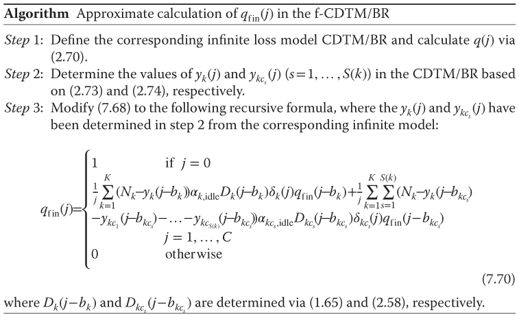
7.9.2.3 An Approximate Algorithm for the Determination of  in the f‐CDTM
The algorithm can be described by the following steps [ 5]:


7.10 The Finite Connection Dependent Threshold Model under the BR Policy
7.10.1 The Service System
In the f‐CDTM under the BR policy (f‐CDTM/BR), ![]() b.u. are reserved to benefit calls of all other service‐classes apart from service‐class k. The application of the BR policy in the f‐CDTM/BR is similar to that of the f‐MTM/BR.
b.u. are reserved to benefit calls of all other service‐classes apart from service‐class k. The application of the BR policy in the f‐CDTM/BR is similar to that of the f‐MTM/BR.
7.10.2 The Analytical Model
7.10.2.1 Link Occupancy Distribution
Based on the Roberts method and the algorithm of Section 7.8.2.1 of the f‐MTM/BR, the unnormalized values of the link occupancy distribution, ![]() , in the f‐CDTM/BR can be determined as follows:
, in the f‐CDTM/BR can be determined as follows:
7.10.2.2 TC Probabilities, CBP, Utilization, and Mean Number of In‐service Calls
Based on (7.70) and (2.58), we can determine the following performance measures:
- The TC probabilities of service‐class k calls with
 b.u.,
b.u.,  , via (6.42).
 - The TC probabilities of service‐class k calls with
 , via:
(7.71)
, via:
(7.71)
- The CC probabilities of service‐class k calls with
 (without the option of
  , via (6.42) but for a system with
  traffic sources.
 - The CC probabilities of service‐class k calls with with
 , via (7.71) but for a system with
  traffic sources.
 - The conditional TC probabilities of service‐class k calls with
 b.u. given that
  , via (7.66), while subtracting the BR parameter
  from
from  .
. - The link utilization,
 , via (6.36).
 - The average number of service‐class k calls in the system accepted with
 b.u.,
b.u.,  , via (6.37) where
  is determined by (7.46).
 - The average number of service‐class k calls in the system accepted with
 b.u.,
b.u.,  , via ( 7.57) where
  is determined by:
(7.72)
is determined by:
(7.72)
7.11 Applications
Since the finite multirate retry‐threshold loss models are a combination of the retry‐threshold loss models of Chapter 2 and the EnMLM of Chapter , the interested reader may refer to Sections 2.11 and 6.5 for possible applications.
7.12 Further Reading
Similar to the previous section, the interested reader may refer to the corresponding section of Chapter 2 (Section 2.12) and Chapter 6 (Section 6.6). In addition to these sections, interesting extensions of the f‐CDTM have been proposed in [7,8], for WCDMA networks. Compared to [ 7], in [ 8], a CAC distinguishes handover traffic from new traffic. More precisely, when the cell load is above a predefined threshold, handover calls are allowed to reduce their bandwidth requirements in order to avoid blocking.
References
- 1 G. Stamatelos and V. Koukoulidis, Reservation‐based bandwidth allocation in a radio ATM network. IEEE/ACM Transactions on Networking, 5(3):420–428, June 1997.
- 2 I. Moscholios, M. Logothetis and P. Nikolaropoulos, Engset multi‐rate state‐dependent loss models. Performance Evaluation, 59(2–3):247–277, February 2005.
- 3 I. Moscholios and M. Logothetis, Engset multirate state‐dependent loss models with QoS guarantee. International Journal of Communication Systems, 19(1):67–93, February 2006.
- 4 I. Moscholios, M. Logothetis and G. Kokkinakis, A simplified blocking probability calculation in the retry loss models for finite sources. Proceedings of Communication Systems, Networks and Digital Signal Processing – 5th CSNDSP, Patras, Greece, July 2006.
- 5 I. Moscholios, M. Logothetis and G. Kokkinakis, On the calculation of blocking probabilities in the multirate state‐dependent loss models for finite sources. Mediterranean Journal of Computers and Networks, 3(3):100–109, July 2007.
- 6 J. Kaufman, Blocking with retrials in a completely shared resource environment. Performance Evaluation, 15(2):99–113, June 1992.
- 7 V. Vassilakis, G. Kallos, I. Moscholios and M. Logothetis, Call‐level analysis of W‐CDMA networks supporting elastic services of finite population. IEEE ICC 2008, Beijing, China, May 2008.
- 8 V. Vassilakis, I. Moscholios, J. Vardakas and M. Logothetis, Handoff modeling in cellular CDMA with finite sources and state‐dependent bandwidth requirements. Proceedings of IEEE CAMAD 2014, Athens, Greece, December 2014.