1
The Erlang Multirate Loss Model
We start with random arriving calls of fixed bandwidth requirements and fixed bandwidth allocation during service.
Before the study of multirate teletraffic loss models where multiple service‐classes of different bandwidth per call requirements are accommodated in a service system, let us begin with the simpler case where all calls belong to just one service‐class, and afterwards consider the multi‐service system.
1.1 The Erlang Loss Model
1.1.1 The Service System
Consider that a single service‐class (e.g., telephone service) is accommodated to a loss system, say a transmission link, of capacity ![]() b.u. Each call arrives in the system according to a Poisson process with mean value
b.u. Each call arrives in the system according to a Poisson process with mean value ![]() and requires 1 b.u. to be serviced. If this bandwidth is available, then a call is accepted in the system and remains under service for an exponentially distributed service time, with mean value
and requires 1 b.u. to be serviced. If this bandwidth is available, then a call is accepted in the system and remains under service for an exponentially distributed service time, with mean value ![]() . Otherwise, when all b.u. are occupied, a call is blocked and lost without further affecting the system (e.g., a blocked call is not allowed to retry).
. Otherwise, when all b.u. are occupied, a call is blocked and lost without further affecting the system (e.g., a blocked call is not allowed to retry).
Now, let ![]() be the number of in‐service calls at the time instant
be the number of in‐service calls at the time instant ![]() . Since each call occupies 1 b.u. then
. Since each call occupies 1 b.u. then ![]() also expresses the number of occupied b.u. at the time instant
also expresses the number of occupied b.u. at the time instant ![]() , i.e.,
, i.e., ![]() . Assume that at time instant
. Assume that at time instant ![]() , (
, (![]() ), the number of in‐service calls is
), the number of in‐service calls is ![]() , that is,
, that is, ![]() ; in the teletraffic jargon, we say that the system is in state
; in the teletraffic jargon, we say that the system is in state ![]() . Let
. Let ![]() denote the probability of being in state
denote the probability of being in state ![]() . Since calls arrive at random, based on (I.10) the system's state becomes
. Since calls arrive at random, based on (I.10) the system's state becomes ![]() at
at ![]() , if one of the following events takes place:
, if one of the following events takes place:
- (a)
 and (no arrival or departure occurs in
  ).
). - (b)
 and (one new call arrives in
  ).
). - (c)
 and (one in‐service call departs from the system in
  ).
).
The probability of the first event equals ![]() . Note that the probability for a specific call to depart within
. Note that the probability for a specific call to depart within ![]() is
is ![]() ; given that there are
; given that there are ![]() in‐service calls, one departure is possible due to the first or the second or the
in‐service calls, one departure is possible due to the first or the second or the ![]() th call, and therefore the probability of one departure becomes the sum of
th call, and therefore the probability of one departure becomes the sum of ![]() probabilities:
probabilities: ![]() .
.
The probability of the second event equals ![]() , while the probability of the last event equals
, while the probability of the last event equals ![]() (because of the
(because of the ![]() in‐service calls).
in‐service calls).
Therefore, because the above events are exclusive, we take:

or

In (1.2), when ![]() , the limit of the LHS defines the derivative of
, the limit of the LHS defines the derivative of ![]() :
:

According to the notion of derivative, (1.3) shows the rate of changes of the instantaneous value of ![]() , which is of little interest. Instead, of great interest is to find the state probability in the steady state, that is, when the system operates normally for a long time period. Service systems normally have a steady state; this means that as
, which is of little interest. Instead, of great interest is to find the state probability in the steady state, that is, when the system operates normally for a long time period. Service systems normally have a steady state; this means that as ![]() . Then, the probability
. Then, the probability ![]() approaches a limiting value
approaches a limiting value ![]() , which is constant over time and is determined through ( 1.3) when the LHS is zero:
, which is constant over time and is determined through ( 1.3) when the LHS is zero:
where ![]() and
and ![]() .
.
Since (1.4) holds for all ![]() , we say that the system is in statistical equilibrium. To find the limiting probabilities
, we say that the system is in statistical equilibrium. To find the limiting probabilities ![]() , also called steady state probabilities, we solve ( 1.4) by applying the so‐called ladder method:
, also called steady state probabilities, we solve ( 1.4) by applying the so‐called ladder method:

By adding these equations side by side, we obtain the following recurrent formula:
where ![]() is the offered traffic‐load in erl.
is the offered traffic‐load in erl.
From (1.5), by successive substitutions, we relate ![]() to the probability that the system is empty,
to the probability that the system is empty, ![]() :
:
One more equation is needed between ![]() and
and ![]() to formulate a system of two equations with two unknowns. Since the system will always be in one of the states
to formulate a system of two equations with two unknowns. Since the system will always be in one of the states ![]() , we have:
, we have:

that is,

By substituting (1.8) to (1.6), we determine ![]() :
:

which is the well‐known Erlang distribution.1
1.1.2 Global and Local Balance
It is important at this point to interpret ( 1.4) and ( 1.5). Let us rewrite them as follows, while multiplying them by ![]() :
:
The LHS of (1.10a) shows the probability sum of two events while the system is in state ![]() : a call arrival (
: a call arrival (![]() ) and a call departure (
) and a call departure (![]() ), which transfer the system out of state
), which transfer the system out of state ![]() , obviously to the adjacent state
, obviously to the adjacent state ![]() or
or ![]() , respectively. Likewise, the RHS of (1.10a) shows the probability of moving to state
, respectively. Likewise, the RHS of (1.10a) shows the probability of moving to state ![]() from the adjacent states
from the adjacent states ![]() and
and ![]() , due to a call arrival and a call departure, respectively. Let us remove
, due to a call arrival and a call departure, respectively. Let us remove ![]() from this equation. Then, (1.10a) denotes the fact that rate‐out = rate‐in and is named the global balance (GB) equation of state
from this equation. Then, (1.10a) denotes the fact that rate‐out = rate‐in and is named the global balance (GB) equation of state ![]() .
.
Even more interesting is the interpretation of (1.10b), where the RHS shows the probability of moving up, from state ![]() to state
to state ![]() , due to a call arrival, while the LHS shows the probability of moving down, from state
, due to a call arrival, while the LHS shows the probability of moving down, from state ![]() to state
to state ![]() , due to a call departure. When removing
, due to a call departure. When removing ![]() , this equation denotes the fact that rate‐down = rate‐up and is named the local balance (LB) equation between the adjacent states
, this equation denotes the fact that rate‐down = rate‐up and is named the local balance (LB) equation between the adjacent states ![]() and
and ![]() .
.
Having removed ![]() from (1.10a), its graphical representation is shown in Figure 1.1 by the state transition diagram of the system. Two LB equations are presented (the first one between states
from (1.10a), its graphical representation is shown in Figure 1.1 by the state transition diagram of the system. Two LB equations are presented (the first one between states ![]() and
and ![]() and the second one between states
and the second one between states ![]() and
and ![]() ). Note at this point that the existence of GB between adjacent states does not guarantee the existence of LB. The opposite holds.
). Note at this point that the existence of GB between adjacent states does not guarantee the existence of LB. The opposite holds.
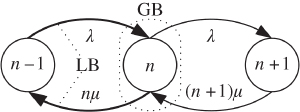
Figure 1.1 State transition diagram for the Erlang loss model ( /
/ /
/ /0).
/0).
Equations (1.10) introduce the following methodology, called classical methodology, in analyzing a service system in equilibrium, i.e., in determining its steady state probabilities:
- (i) Start with the state transition diagram of the system.
- (ii) Write the GB equations.
- (iii) Apply the ladder method to the GB equations in order to obtain simpler equations, usually the LB equations.
- (iv) If steps (ii) and (iii) are too complicated, assume that LB equations hold and go on, but check for atopy.
- (v) Consider the normalization condition.2
- (vi) Solve the resultant linear system of equations of the steady state probabilities.

Figure 1.2  /
/ /
/ /
/ FIFO – state transition diagram for
  (Example 1.2).
1.1.3 Call Blocking Probability
The most3 important question in a loss system is “What is the CBP?” or, equivalently, “What is the GoS?”. Call blocking occurs when the system is fully occupied, that is, CBP equals ![]() , the probability that the system is in state
, the probability that the system is in state ![]() . From ( 1.9) we have
. From ( 1.9) we have

Equation (1.22) is the famous Erlang‐B formula also met in (I.5). As we discussed there (Example I.5), the closed form of the Erlang‐B formula is not appealing for large values of ![]() and
and ![]() , instead its recurrent form (I.8) is not only preferred but necessary.
, instead its recurrent form (I.8) is not only preferred but necessary.
It is worth mentioning at this point that, as has been investigated (e.g., [1–3]), ( 1.9) and consequently ( 1.22) are insensitive to the distribution of service time, and depend only on the mean holding time, ![]() , which is inherently included in the traffic‐load (
, which is inherently included in the traffic‐load (![]() ). Besides, ( 1.22) refers to the proportion of time that all
). Besides, ( 1.22) refers to the proportion of time that all ![]() b.u. are occupied (i.e., the system is congested). This probability is named time congestion (TC) probability and can be measured by an outside observer. Due to the PASTA property, an inside observer sees the same probability, therefore ( 1.22) is also called call congestion (CC) probability or CBP.
b.u. are occupied (i.e., the system is congested). This probability is named time congestion (TC) probability and can be measured by an outside observer. Due to the PASTA property, an inside observer sees the same probability, therefore ( 1.22) is also called call congestion (CC) probability or CBP.
Having found a relationship between ![]() ,
, ![]() and GoS, i.e.,
and GoS, i.e., ![]() , let us now provide graphs of them (Figure 1.3) in order to compare them with the qualitative graphs of Figure I.2. The first graph of Figure 1.3 presents the required system capacity
, let us now provide graphs of them (Figure 1.3) in order to compare them with the qualitative graphs of Figure I.2. The first graph of Figure 1.3 presents the required system capacity ![]() versus the offered traffic‐load
versus the offered traffic‐load ![]() (for two certain values of GoS: 1% and 3%) and corresponds to the LHS graph of Figure I.2. However, the anticipated curve of Figure I.2 is hardly followed in Figure 1.3; the function
(for two certain values of GoS: 1% and 3%) and corresponds to the LHS graph of Figure I.2. However, the anticipated curve of Figure I.2 is hardly followed in Figure 1.3; the function ![]() is rather a straight line in a wide range of the presented values of traffic‐load. The second graph of Figure 1.3 presents CBP versus
is rather a straight line in a wide range of the presented values of traffic‐load. The second graph of Figure 1.3 presents CBP versus ![]() , for
, for ![]() erl and
erl and ![]() erl, and corresponds to the middle graph of Figure I.2. Due to the reverse meaning of CBP,4 the convex curvature of the middle graph in Figure I.2 appears in the middle graph of Figure 1.3, as a concave (reverse) curvature. The third graph of Figure 1.3 presents CBP versus traffic‐load
erl, and corresponds to the middle graph of Figure I.2. Due to the reverse meaning of CBP,4 the convex curvature of the middle graph in Figure I.2 appears in the middle graph of Figure 1.3, as a concave (reverse) curvature. The third graph of Figure 1.3 presents CBP versus traffic‐load ![]() for two values of
for two values of ![]() : 5 and 6 b.u. Herein, the corresponding qualitative graph of Figure I.2 (RHS) is followed pretty well.
: 5 and 6 b.u. Herein, the corresponding qualitative graph of Figure I.2 (RHS) is followed pretty well.

Figure 1.3 Quantitative relationships between traffic‐load, system capacity, and CBP.
1.1.4 Other Performance Metrics
- Utilization: The utilization,
 , is expressed by the average number of occupied b.u.:
(1.24)
, is expressed by the average number of occupied b.u.:
(1.24)
Equation (1.24) verifies (I.34). Because of property (4) of traffic‐load,
 .
. - Trunk efficiency: According to (I.35), the trunk efficiency
 is:
(1.25)
is:
(1.25)
Since
 expresses traffic‐load per trunk,
  (property (3) of traffic‐load). Thus, again,
  . As Figure 1.4 shows, the trunk efficiency increases as the system capacity increases, for a certain GoS. This is called the large‐scale effect and leads to the conclusion that loss systems must be designed with the greatest possible capacity in order for trunks to be used efficiently. The latter happens because the larger the system capacity, the greater the carried traffic conveyed under a certain GoS.

Figure 1.4 Trunk efficiency for various values of GoS and  .
.
- A low bound of
 : Since
  always, we have:
(1.26)
always, we have:
(1.26)
Equation (1.26) can be used for a fast evaluation of CBP measurements or CBP calculations, given that the offered traffic‐load
 estimation is correct. For instance, according to ( 1.26), if
  b.u. and
  erl, the anticipated CBP
  % at least. Note that the actual CBP value is
  . The interested reader may resort to [4] and the references therein for an in‐depth analysis of the lower and upper bounds on the Erlang‐B and Erlang‐C formulas.
1.2 The Erlang Multirate Loss Model
1.2.1 The Service System
Let us now consider the multi‐service system or, as we call it, the Erlang multirate loss model (EMLM). A single link of capacity ![]() b.u. accommodates calls of
b.u. accommodates calls of ![]() different service‐classes under the CS policy. Each call of service‐class
different service‐classes under the CS policy. Each call of service‐class ![]() arrives in the system following a Poisson process with mean rate
arrives in the system following a Poisson process with mean rate ![]() and requires
and requires ![]() b.u. to be serviced. If the requested bandwidth is available, then a call is accepted in the system and remains under service for an exponentially distributed service time, with mean
b.u. to be serviced. If the requested bandwidth is available, then a call is accepted in the system and remains under service for an exponentially distributed service time, with mean ![]() . Otherwise, the call is blocked and lost, without further affecting the system. After service completion, the
. Otherwise, the call is blocked and lost, without further affecting the system. After service completion, the ![]() b.u. are released and become available to new arriving calls.
b.u. are released and become available to new arriving calls.
Let ![]() denote the number of in‐service calls of service‐class
denote the number of in‐service calls of service‐class ![]() in the steady state,
in the steady state, ![]() ) the corresponding vector of all in‐service calls of all service‐classes, and
) the corresponding vector of all in‐service calls of all service‐classes, and ![]() ) the corresponding vector of the required bandwidth per call of all service‐classes in the system. Because of the CS policy, the set
) the corresponding vector of the required bandwidth per call of all service‐classes in the system. Because of the CS policy, the set ![]() of the system (state space) is given by (I.36). The product
of the system (state space) is given by (I.36). The product ![]() expresses the occupied link bandwidth in system state
expresses the occupied link bandwidth in system state ![]() and plays a decisive role in CAC:
and plays a decisive role in CAC:
In terms of ![]() , the CAC is expressed as follows. A new call of service‐class
, the CAC is expressed as follows. A new call of service‐class ![]() that finds the system in state
that finds the system in state ![]() is accepted in the system if
is accepted in the system if ![]() , where
, where ![]() .
.
In any case, the best way to prove that a system has a PFS,5 is to find it!
1.2.2 The Analytical Model
1.2.2.1 Steady State Probabilities
In analyzing a service system, the first target is to determine the steady state probability ![]() . For the EMLM, it can be determined, obviously, by extending the PFS (1.29) of Example 1.6 to
. For the EMLM, it can be determined, obviously, by extending the PFS (1.29) of Example 1.6 to ![]() service‐classes, as follows:
service‐classes, as follows:

where ![]() the normalization constant, which is determined through
the normalization constant, which is determined through ![]() :
:

Of course, the PFS (1.30) must satisfy the set of GB and LB equations of the system. To verify it, follow the aforementioned classical methodology:
- (i)
Draw the state transition diagram and write the GB equations. Figure 1.7 shows the one‐dimensional state transition diagram of the EMLM when a general state
 is considered. Normally, the state transition diagram has as many dimensions (axes) as the number of service‐classes
  ; see the LHS of Figure 1.8. To be converted to a one‐dimensional diagram, we define the equivalent diagram at the RHS of Figure 1.8. This consideration is justified because both diagrams lead to the same GB equation (see 1.32). Thus, the GB equation (rate in = rate out) for state
  is given by:
(1.32)where
is given by:
(1.32)where
 are the probability distributions of the corresponding states
  ; parameters
  validate a state transition through the following expressions:
(1.33)
validate a state transition through the following expressions:
(1.33)

Figure 1.7 State transition diagram of the EMLM.

Figure 1.8 GB in the system of Example 1.6 (Example 1.7).
- (ii) Assume that LB exists and check for atopy.
Assuming the existence of LB between any adjacent states (
 and
and  , or
, or  and
and  , for
, for  ), then the following LB equations (rate up = rate down) are extracted from the state transition diagram (Figure 1.8, LHS) (correspondingly):(1.34a)
 (1.34b)
- (iii) Solve the resultant linear system of equations of the equilibrium probabilities, while considering the normalization condition. Check for atopy, again.
It can be verified that the probability distribution
 has a PFS by substituting ( 1.30) into (1.34a) or (1.34b).
Having calculated the steady state probability ![]() , we proceed to determine the CBP. To this end, we denote by
, we proceed to determine the CBP. To this end, we denote by ![]() the admissible state space of service‐class
the admissible state space of service‐class ![]() :
: ![]() . A new service‐class
. A new service‐class ![]() call is accepted in the system, if, at the time point of its arrival, the system is in a state
call is accepted in the system, if, at the time point of its arrival, the system is in a state ![]() . Hence, the CBP of service‐class
. Hence, the CBP of service‐class ![]() is determined by the state space
is determined by the state space ![]() , as follows:
, as follows:

Equation ( 1.35) provides the CBP of the EMLM based on a PFS. A recurrent form for the CBP calculation can be obtained by expressing ( 1.36), as follows:

where ![]() ; the values of
; the values of ![]() can be determined recursively via:
can be determined recursively via:

For large values of ![]() the computational complexity of (1.38) is
the computational complexity of (1.38) is ![]() 6. A simpler formula follows with a computational complexity
6. A simpler formula follows with a computational complexity ![]() ,7 for the determination of the state probabilities of the system, when the system state is represented not by the number of in‐service calls of each service‐class, but by the total occupied b.u.
,7 for the determination of the state probabilities of the system, when the system state is represented not by the number of in‐service calls of each service‐class, but by the total occupied b.u. ![]() in the link, where
in the link, where ![]() . This state representation is more effective when aimed at calculating the key performance metrics of the system, like CBP and link utilization. The unnormalized values
. This state representation is more effective when aimed at calculating the key performance metrics of the system, like CBP and link utilization. The unnormalized values ![]() of the link occupancy distribution, i.e., the probability that
of the link occupancy distribution, i.e., the probability that ![]() out of
out of ![]() b.u. are occupied, are given by:
b.u. are occupied, are given by:

Equation (1.39), known in the literature as the Kaufman–Roberts8 recursion, is accurate and computationally efficient with an easy computer implementation. Because of this, it is the springboard to derive other more complex but efficient teletraffic models. In order for the ![]() values of ( 1.39) to become probabilities, they must be normalized through division by the sum of them,
values of ( 1.39) to become probabilities, they must be normalized through division by the sum of them, ![]() :
:

Note that ![]() denotes either a normalized or unnormalized value of the link occupancy distribution, but, in any case, it will be explicitly mentioned (unless it is clear), while
denotes either a normalized or unnormalized value of the link occupancy distribution, but, in any case, it will be explicitly mentioned (unless it is clear), while ![]() denotes a normalized value of the link occupancy distribution.
denotes a normalized value of the link occupancy distribution.
Proof of ( 1.39): According to [5], let us consider the occupied link bandwidth ![]()
![]() , as a system state. Thus, the system can be seen either via state
, as a system state. Thus, the system can be seen either via state ![]() (multi‐dimensional system) or via the new (aggregate) state
(multi‐dimensional system) or via the new (aggregate) state ![]() (one‐dimensional system). The link occupancy distribution
(one‐dimensional system). The link occupancy distribution ![]() is defined as:
is defined as:

where ![]() is the set of states in which exactly
is the set of states in which exactly ![]() b.u. are occupied by all in‐service calls:
b.u. are occupied by all in‐service calls: ![]() (Figure 1.9).
(Figure 1.9).

Figure 1.9 Sets  and
and  for the EMLM of two service‐classes, under the CS policy.
The key point for the recursive calculation of ![]() is to associate the values of
is to associate the values of ![]() values with the “previous” values of
values with the “previous” values of ![]() . In other words, we have to relate the values of
. In other words, we have to relate the values of ![]() with the (“previous”) values of
with the (“previous”) values of ![]() , since in state
, since in state ![]() there are
there are ![]() in‐service calls of service‐class
in‐service calls of service‐class ![]() , while in state
, while in state ![]() there are
there are ![]() in‐service calls (assuming that
in‐service calls (assuming that ![]() ). This relation will be achieved by the use of the LB equation (1.34a), as we will shortly show.
). This relation will be achieved by the use of the LB equation (1.34a), as we will shortly show.
Since ![]() , we can write (1.41) as follows:
, we can write (1.41) as follows:
From the LB equation (1.34a), the product ![]() is determined by:
is determined by:

where the parameter ![]() is replaced by
is replaced by ![]() (another binary parameter) to denote that:
(another binary parameter) to denote that:

We take sums of both sides of (1.43) over ![]() to have:
to have:

Equation ( 1.43) has no meaning when ![]() ; since the RHS of (1.45) refers to state
; since the RHS of (1.45) refers to state ![]() , the previous state
, the previous state ![]() (in which the LHS of ( 1.45) refers to) belongs to
(in which the LHS of ( 1.45) refers to) belongs to ![]() given that
given that ![]() . This is expressed through the parameters
. This is expressed through the parameters ![]() . More formally, when
. More formally, when ![]() , the LHS of ( 1.45) is written as:
, the LHS of ( 1.45) is written as:

and the set ![]() defines the state space
defines the state space ![]() . To individuate the case where
. To individuate the case where ![]() , we introduce the following variable:
, we introduce the following variable:

By using (1.47), and because of the definition ( 1.41), we can write (1.46) as follows:

From ( 1.45), ( 1.46), and (1.48), we obtain:

Based on (1.49), (1.42) is written as:

which is the Kaufman–Roberts recursion ( 1.39). For an alternative proof see Example 1.12.
Q.E.D.
According to [ 5], ( 1.39) can be used for arbitrary distributed service times. An interesting interpretation of ( 1.39) is that it stands for an LB equation of a birth–death process, in which ![]() is the birth rate of service‐class
is the birth rate of service‐class ![]() calls,
calls, ![]() is the corresponding death rate, and
is the corresponding death rate, and ![]() is the mean number of service‐class
is the mean number of service‐class ![]() calls in state
calls in state ![]() (Figure 1.10):
(Figure 1.10):
Indeed, (1.51) is derived from ( 1.49) because the RHS of ( 1.49) is written as follows:
Note that ( 1.39) can be derived from ( 1.51) by multiplying both sides of ( 1.51) by ![]() and summing over
and summing over ![]() .
.

Figure 1.10 The Kaufman–Roberts recursion as a birth–death process.
1.2.2.2 CBP, Utilization, and Mean Number of In‐service Calls
The following performance measures are determined based on ( 1.39):
- CBP: The determination of CBP of service‐class
 , is given by:
(1.53)
, is given by:
(1.53)
where
 is given by (1.40).
Figure 1.11 depicts a helpful visualization regarding (1.53).

Figure 1.11 Visualization of CBP calculation.
Note that ( 1.53) refers to the TC probabilities of service‐class
 calls. These probabilities coincide with the CBP due to the PASTA property.
Needless to say that in the case of one service‐class in the system, the CBP obtained by ( 1.53) coincides with the results of the Erlang‐B formula; hence, we name this model the Erlang multirate loss model.
- Utilization: The link utilization,
 , is calculated by:
(1.54)
, is calculated by:
(1.54)
- Mean number of in‐service calls in state
 : The mean number of in‐service calls of service‐class
  in state
  is given (because of ( 1.51)) by:
(1.55)
is given (because of ( 1.51)) by:
(1.55)
Note that
 , if
, if  .
. - Mean number of in‐service calls in the system: The mean number of in‐service calls for service‐class
 in the system,
  , is given by:
(1.56)
, is given by:
(1.56)

Figure 1.12 CBP oscillations in the EMLM (CS policy) (Example 1.14).
1.3 The Erlang Multirate Loss Model under the BR policy
1.3.1 The Service System
We consider again the multi‐service system of the EMLM, but with the following CAC. A new service‐class ![]() call is accepted in the link if, after its acceptance, the link has at least
call is accepted in the link if, after its acceptance, the link has at least ![]() b.u. available to serve calls of other service‐classes. This service system is called EMLM under the BR policy (EMLM/BR). By properly selecting the BR parameters
b.u. available to serve calls of other service‐classes. This service system is called EMLM under the BR policy (EMLM/BR). By properly selecting the BR parameters ![]() , we can achieve CBP equalization among service‐classes; this is the main target of the BR policy. Assuming that
, we can achieve CBP equalization among service‐classes; this is the main target of the BR policy. Assuming that ![]() , then for CBP equalization the parameters
, then for CBP equalization the parameters ![]() are chosen so that
are chosen so that ![]() , that is,
, that is, ![]() , since it is reasonable not to reserve bandwidth against the service‐class which requires the maximum bandwidth per call. Obviously, due to CBP equalization, we avoid the CBP oscillations observed in the EMLM under the CS policy.
, since it is reasonable not to reserve bandwidth against the service‐class which requires the maximum bandwidth per call. Obviously, due to CBP equalization, we avoid the CBP oscillations observed in the EMLM under the CS policy.
Figure 1.13 illustrates the case of a single link with ![]() that accommodates calls of two service‐classes with
that accommodates calls of two service‐classes with ![]() and
and ![]() b.u. To achieve CBP equalization we reserve
b.u. To achieve CBP equalization we reserve ![]() b.u. in favor of calls of the second service‐class.
b.u. in favor of calls of the second service‐class.

Figure 1.13 An example of the EMLM under the BR policy.
1.3.2 The Analytical Model
The basic characteristic of the BR policy is that the steady state probabilities cannot be calculated via a PFS. This is because LB between some adjacent states is destroyed (see the following example).
1.3.2.1 Accurate CBP Calculation
The absence of a PFS in the EMLM/BR leads to approximate solutions as far as the recursive calculation of the state probabilities (and consequently the CBP) is concerned. An accurate CBP calculation is achieved only by solving the linear system of GB equations; however, this is applicable only to small systems with a few service‐classes. Otherwise, the computational requirements become quite excessive.
1.3.2.2 Approximate CBP Calculation based on the Roberts Method
In the EMLM/BR, the link occupancy distribution, q(j), is given in an approximate way by the following recursive formula [11]:

where:

This formula has a form similar to the Kaufman–Roberts recursion ( 1.39), and its existence is based on the assumption that, for a service‐class ![]() with
with ![]() , the mean number of service‐class
, the mean number of service‐class ![]() calls in state
calls in state ![]() ,
, ![]() , is zero in all states
, is zero in all states ![]() which belong to the prohibitive space of this service‐class:
which belong to the prohibitive space of this service‐class: ![]() . Thanks to this assumption, which is reflected in the variable
. Thanks to this assumption, which is reflected in the variable ![]() , the one‐dimensional Markov chain of the system is transformed to an approximate reversible Markov chain,9 which leads to the recurrent formula (1.64). Markov chain reversibility is a strong indication of the existence of a PFS.
, the one‐dimensional Markov chain of the system is transformed to an approximate reversible Markov chain,9 which leads to the recurrent formula (1.64). Markov chain reversibility is a strong indication of the existence of a PFS.
The CBP of service‐class ![]() ,
, ![]() , is given by:
, is given by:

where ![]() is the normalization constant, given by ( 1.40).
is the normalization constant, given by ( 1.40).
The link utilization, ![]() , is given by ( 1.54).
, is given by ( 1.54).
The mean number of service‐class ![]() calls, in state
calls, in state ![]() , is determined by:
, is determined by:

The mean number of service‐class ![]() calls in the system,
calls in the system, ![]() , is given by ( 1.56).
, is given by ( 1.56).

Figure 1.15 The one‐dimensional Markov chain of the EMLM/BR (Roberts' assumption, Example 1.18) .
1.3.2.3 CBP Calculation Recursively based on the Stasiak–Glabowski Method
When aiming at QoS equalization among service‐classes, the recursive CBP calculation of the EMLM/BR according to the Roberts method can be improved by the following method proposed by Stasiak and Glabowski10 [12]. The average number of service‐class ![]() calls,
calls, ![]() , in state
, in state ![]() is not zero but positive, and can be determined approximately in a recurrent way by:
is not zero but positive, and can be determined approximately in a recurrent way by:

where for the calculation of ![]() the corresponding EMLM system under the CS policy is assumed (i.e., the Kaufman–Roberts recursion ( 1.39)), while
the corresponding EMLM system under the CS policy is assumed (i.e., the Kaufman–Roberts recursion ( 1.39)), while ![]() is a weight given by:
is a weight given by:

The weight ![]() determines the proportion of
determines the proportion of ![]() that is transferred in state
that is transferred in state ![]() by a call of service‐class
by a call of service‐class ![]() (other than
(other than ![]() ), assuming that
), assuming that ![]() . Although the system cannot be in state
. Although the system cannot be in state ![]() due to an arriving call of service‐class
due to an arriving call of service‐class ![]() (because of the BR policy), the system can be in state
(because of the BR policy), the system can be in state ![]() due to arriving calls of other service‐classes (calls of other service‐classes may coexist in previous states together with service‐class
due to arriving calls of other service‐classes (calls of other service‐classes may coexist in previous states together with service‐class ![]() calls). Thus, when the system is transferred to state
calls). Thus, when the system is transferred to state ![]() by a service‐class
by a service‐class ![]() call, this call also transfers to state
call, this call also transfers to state ![]() the population of service‐class
the population of service‐class ![]() . Therefore, the assumption that the average number of calls is positive even in a prohibitive state of a service‐class is more realistic compared to the Roberts assumption. Figure 1.16 illustrates the fact that calls from different service‐classes may contribute in transferring the population of service‐class
. Therefore, the assumption that the average number of calls is positive even in a prohibitive state of a service‐class is more realistic compared to the Roberts assumption. Figure 1.16 illustrates the fact that calls from different service‐classes may contribute in transferring the population of service‐class ![]() to a prohibitive state
to a prohibitive state ![]() . Consequently, given that in state
. Consequently, given that in state ![]() the population of service‐class
the population of service‐class ![]() does exist, a backward transition to state
does exist, a backward transition to state ![]() is true.
is true.

Figure 1.16 Calls of service‐classes  contribute in
  by transferring the population of service‐class
  to state
  .
.
Having determined the average number of calls in each state ![]() via (1.68), then the Roberts method is followed by replacing
via (1.68), then the Roberts method is followed by replacing ![]() in the RHS of
in the RHS of ![]() in ( 1.64) by
in ( 1.64) by ![]() , in order for the average number of calls of each service‐class in state
, in order for the average number of calls of each service‐class in state ![]() to be determined:
to be determined:

The philosophy behind this method is that the approximated reversible Markov chain of the Roberts method is kept, but each state ![]() of the prohibited state space is now substituted by state
of the prohibited state space is now substituted by state ![]() . The Stasiak–Glabowski method is summarized in the following procedure:
. The Stasiak–Glabowski method is summarized in the following procedure:
- Step 1:
Assuming that the system is under the CS policy (instead of the BR policy), calculate
 via ( 1.39).
 - Step 2:
Calculate the average number of service‐class
 calls in state
  ,
,  , according to ( 1.68) and (1.69).
 - Step 3: Determine
 for the EMLM/BR, as follows:
(1.71)
for the EMLM/BR, as follows:
(1.71)
- Step 4: Determine the CBP of each service‐class according to ( 1.66).
1.4 The Erlang Multirate Loss Model under the Threshold Policy
1.4.1 The Service System
We consider again the multi‐service system of the EMLM and adopt a TH‐type CAC, as follows: A new call of service‐class k is accepted in the system, of C b.u., if:
- (i) its bandwidth requirement, bk b.u., is less or equal to the available link bandwidth
- (ii) the number nk of in‐service calls of service‐class k does not exceed a predefined threshold parameter, after its acceptance. Otherwise, the call is blocked and lost without affecting the system.
By definition a policy is called a TH policy if there exists a set of positive integers ![]() such that a service‐class
such that a service‐class ![]() call is accepted in the system when in state
call is accepted in the system when in state ![]() , if and only if the new system state fulfils the relations
, if and only if the new system state fulfils the relations ![]() and
and ![]() [13].
[13].
1.4.2 The Analytical Model
1.4.2.1 Steady State Probabilities
Due to the fact that the TH policy is a coordinate convex policy (as the CS policy is) the steady state probabilities in the EMLM/TH have a PFS whose form is the same as that of the EMLM (only the definition of ![]() differs):
differs):

where ![]() and
and ![]()
For the determination of the unnormalized values of q(j), the following accurate and recursive formula can be used [14]:

where ![]() is the probability that
is the probability that ![]() b.u. are occupied, while the number of service‐class
b.u. are occupied, while the number of service‐class ![]() calls is
calls is ![]() or:
or:
In (1.73) the fact that ![]() implies that:
implies that:
- (i)
 and therefore
  for
for  and
and - (ii)
 is a blocking probability factor for service‐class
  calls.
The proof of ( 1.73) is similar to the proof of the Kaufman–Roberts formula (see e.g., [ 14]). The only difference is that ( 1.48) now takes the form:

due to the existence of the TH policy.
Intuitively, the form of (1.75) is expected, since the term ![]() is a factor that blocks a new service‐class
is a factor that blocks a new service‐class ![]() call from being accepted in the system and therefore blocks the transition from state
call from being accepted in the system and therefore blocks the transition from state ![]() to state
to state ![]() .
.
1.4.2.2 CBP, Utilization and Mean Number of In‐service Calls
The following performance measures can be determined:
- To determine the CBP of service‐class
 ,
,  , we consider two groups of macro‐states:
- (i)
those where there is no available bandwidth to accept a new service‐class
 call; this happens when
- (ii)
those where available bandwidth exists, i.e.,
 but
but  ; the latter implies that
  .
.
The values of
 are given by:(1.76)
where
 is the normalization constant.
 - (i)
those where there is no available bandwidth to accept a new service‐class
- The link utilization is given by ( 1.54).
- The mean number
 of service‐class
  calls, in state
  , is given by:
(1.77)
, is given by:
(1.77)
- The mean number of service‐class
 calls in the system is given by ( 1.56).
Equations (1.76) and (1.77) require knowledge of ![]() . The latter takes positive values when
. The latter takes positive values when ![]() . Thus, we consider a subsystem of capacity
. Thus, we consider a subsystem of capacity ![]() that accommodates all service‐classes but service‐class
that accommodates all service‐classes but service‐class ![]() . For this subsystem, we define
. For this subsystem, we define ![]() , which is analogous to
, which is analogous to ![]() of ( 1.73):
of ( 1.73):

We can now compute ![]() for
for ![]() , as follows:
, as follows:

In (1.79), the term ![]() is expected, since for states
is expected, since for states ![]() , the number of in‐service calls of service‐class
, the number of in‐service calls of service‐class ![]() is always
is always ![]() .
.
The computational complexity of the EMLM/TH is in the order of ![]() , where
, where ![]() ; for more details, see [ 14].
; for more details, see [ 14].
Note: In (1.78), each time that the calculation of ![]() requires knowledge of
requires knowledge of ![]() (this happens when
(this happens when ![]() , for
, for ![]() , an extra subsystem is needed for the calculation of
, an extra subsystem is needed for the calculation of ![]() and
and ![]() via ( 1.78) and ( 1.79) (see also Section IV, pp. 12–69 in [ 14]). Instead of using subsystems, we may calculate
via ( 1.78) and ( 1.79) (see also Section IV, pp. 12–69 in [ 14]). Instead of using subsystems, we may calculate ![]() for those values of
for those values of ![]() that result in
that result in ![]() (in ( 1.78)), while for the rest values of
(in ( 1.78)), while for the rest values of ![]() we can use the following formula (which is based on the fact that the EMLM/TH has a PFS):
we can use the following formula (which is based on the fact that the EMLM/TH has a PFS):

for ![]() and
and ![]() .
.
This method can be useful especially for systems with small to moderate state spaces (see Example 3.10). This topic remains open to investigation.
1.5 The Erlang Multirate Loss Model in a Fixed Routing Network
1.5.1 The Service System
According to ITU‐T, a fixed routing network is a network in which a route11 providing a connection between an originating node and a destination node is fixed for every service‐class (or for every traffic flow of the same service‐class). Let us consider that a fixed routing network consists of ![]() links. Each link
links. Each link ![]() has a fixed capacity of
has a fixed capacity of ![]() b.u. The network accommodates calls of
b.u. The network accommodates calls of ![]() service‐classes under the CS policy. Calls of service‐class
service‐classes under the CS policy. Calls of service‐class ![]() follow a Poisson process with rate
follow a Poisson process with rate ![]() , require
, require ![]() b.u. and have a generally distributed service time with mean
b.u. and have a generally distributed service time with mean ![]() . Let
. Let ![]() be the fixed route of service‐class
be the fixed route of service‐class ![]() calls in the network, where
calls in the network, where ![]() . A call of service‐class
. A call of service‐class ![]() is accepted in the network if its
is accepted in the network if its ![]() b.u. are available in every link
b.u. are available in every link ![]() , otherwise the call is blocked and lost.
, otherwise the call is blocked and lost.
1.5.2 The Analytical Model
Let ![]() be the number of in‐service calls of service‐class
be the number of in‐service calls of service‐class ![]() in the steady state of the system and
in the steady state of the system and ![]() be the corresponding steady state vector of all service‐classes in the fixed routing network. If
be the corresponding steady state vector of all service‐classes in the fixed routing network. If ![]() is the set of service‐classes whose calls are accommodated in link
is the set of service‐classes whose calls are accommodated in link ![]() , i.e.,
, i.e., ![]() , then the state space
, then the state space ![]() of the system is given by:
of the system is given by:

1.5.2.1 Steady State Probabilities
The steady state probabilities ![]() have a PFS whose form is the following [ 13,15]:
have a PFS whose form is the following [ 13,15]:
where  is the normalization constant, and
 ![]() is the offered traffic‐load of service‐class
is the offered traffic‐load of service‐class ![]() calls.
calls.
If we denote by ![]() the occupied b.u. of link
the occupied b.u. of link ![]() , where
, where ![]() , and
, and ![]() is the corresponding vector of the entire fixed routing network, then the unnormalized values of the occupancy distribution
is the corresponding vector of the entire fixed routing network, then the unnormalized values of the occupancy distribution ![]() in the fixed routing network are given by the following L‐dimensional accurate recursive formula [ 15]:
in the fixed routing network are given by the following L‐dimensional accurate recursive formula [ 15]:

where 
![]() is the
is the ![]() th row of a (
th row of a (![]() ) matrix (routing table), and shows the route (sequence of links) for the
) matrix (routing table), and shows the route (sequence of links) for the ![]() th service‐ class.
th service‐ class.
Note: In the case of a single link, (1.83) becomes the Kaufman–Roberts recursion ( 1.39).
1.5.2.2 CBP, Utilization, and Mean Number of In‐service Calls in the System
Having determined the values of ![]() , the following performance measures can be determined:
, the following performance measures can be determined:
- We calculate the CBP of service‐class
 , as follows:
(1.84)where
, as follows:
(1.84)where
 .
. - The utilization of link
 , is given by the following formula:
(1.85)where
, is given by the following formula:
(1.85)where
 .
. - The mean number of service‐class k calls in state
 ,
,  , is determined by the formula:
(1.86)
, is determined by the formula:
(1.86)
- The mean number of service‐class k calls in the system,
 , is given by:
(1.87)
, is given by:
(1.87)
Although ( 1.83) determines CBP in an accurate way, it has a high computational complexity of the order ![]() [16]. The latter shows the necessity for approximate methods that can be used instead of ( 1.83), especially in the case of large networks. The most popular method is the reduced load approximation (RLA) (see e.g., [ 13, 15,17], and [18]) and is the subject of the next subsection.
[16]. The latter shows the necessity for approximate methods that can be used instead of ( 1.83), especially in the case of large networks. The most popular method is the reduced load approximation (RLA) (see e.g., [ 13, 15,17], and [18]) and is the subject of the next subsection.
1.5.3 CBP Calculation by the RLA Method
1.5.3.1 A Fixed Routing Network Supporting a Single Service‐class
We assume that a fixed routing network supports K different traffic flows of a single service‐class requiring 1 b.u. per traffic flow, that is, ![]() . Traffic flows are distinguished by the different sequence of links traversing the various end‐to‐end connections in a fixed routing network. Let
. Traffic flows are distinguished by the different sequence of links traversing the various end‐to‐end connections in a fixed routing network. Let ![]() be the total offered traffic‐load to a link
be the total offered traffic‐load to a link ![]() , where
, where ![]() :
:

where ![]() is the set of traffic flows utilizing link
is the set of traffic flows utilizing link ![]() .
.
The CBP of traffic‐flow ![]() , can be upper bounded by the following product (based on the Erlang‐B formula) [19]:
, can be upper bounded by the following product (based on the Erlang‐B formula) [19]:

This product‐bound provides a good CBP approximation only if the number of links used by traffic flows in the network is small. If not, this bound is unreliable, for example consider only one traffic flow traversing ![]() links of the same capacity
links of the same capacity ![]() . Then, from (1.89), we have [ 13]:
. Then, from (1.89), we have [ 13]:
where ![]() for every link
for every link ![]() .
.
The bound of (1.90) approaches unity when ![]() increases, although
increases, although ![]() for every link and, consequently, for the entire fixed routing network.
for every link and, consequently, for the entire fixed routing network.
A better CBP approximation is achieved by reducing the offered traffic‐load ![]() so that blocking in the other links (excluding
so that blocking in the other links (excluding ![]() ) is taken into account. Specifically, this is done by substituting in (1.88) the term
) is taken into account. Specifically, this is done by substituting in (1.88) the term ![]() with
with ![]() , where the reduced factor
, where the reduced factor ![]() is the probability that there is at least 1 b.u. available in every link of the route
is the probability that there is at least 1 b.u. available in every link of the route ![]() . Denoting the approximate CBP in link
. Denoting the approximate CBP in link ![]() by
by ![]() , we obtain:
, we obtain:

Assuming that blocking is independent from link to link (an assumption that is incorrect), we have [ 13]:

The combination of (1.91) and (1.92) gives the following fixed‐point equation12 for the approximate CBP determination in link l:

Assuming again that blocking is independent from link to link, we approximate the CBP of traffic flow k, ![]() , as follows [ 13]:
, as follows [ 13]:

The combination of (1.93) and (1.94) constitutes the RLA method (or the so‐called Erlang fixed point equation, see e.g., [20]) for fixed routing networks that support traffic flows of a single service‐class.
Note that the fixed point equation has a unique solution (see e.g., Theorem 5.9 in [ 13]) which satisfies the bound:

This solution can be obtained via a simple method that relies on repeated substitutions, as the following example shows.

Figure 1.24 Application of the RLA method in a telephone network of three links (Example 1.26).
1.5.3.2 A Fixed Routing Network Supporting Multiple Service‐classes
Consider now that ![]() service‐classes are accommodated in a fixed routing network of
service‐classes are accommodated in a fixed routing network of ![]() links, according to the service system described in Section 1.5.1. Suppose that a service‐class
links, according to the service system described in Section 1.5.1. Suppose that a service‐class ![]() traverses a link
traverses a link ![]() of capacity
of capacity ![]() b.u. and experiences there CBP,
b.u. and experiences there CBP, ![]() .
. ![]() can be determined approximately by:
can be determined approximately by:

where it is assumed that the offered traffic‐load ![]() of service‐class
of service‐class ![]() to the whole fixed routing network is the same as the offered traffic‐load of service‐class
to the whole fixed routing network is the same as the offered traffic‐load of service‐class ![]() in link
in link ![]() ;
; ![]() is the unnormalized probability of having
is the unnormalized probability of having ![]() occupied b.u. in this link (calculated by the Kaufman–Roberts recursion, ( 1.39), over all
occupied b.u. in this link (calculated by the Kaufman–Roberts recursion, ( 1.39), over all ![]() ) and
) and ![]() is the corresponding normalization constant.
is the corresponding normalization constant.
The CBP expression (1.96) can be improved by considering that the offered traffic‐load of a service‐class to a link is actually reduced when traversing through a sequence of links. Let us denote by ![]() the improved CBP of service‐class
the improved CBP of service‐class ![]() in link
in link ![]() . Based on ( 1.92), the offered traffic‐load
. Based on ( 1.92), the offered traffic‐load ![]() is reduced to
is reduced to ![]() . Then,
. Then, ![]() is given by [ 13]:
is given by [ 13]:

Based on (1.97), the approximate CBP calculation of service‐ class ![]() , in the entire route
, in the entire route ![]() , is given by:
, is given by:

The combination of ( 1.97) and (1.98) constitutes the RLA method for fixed routing networks that support calls of different service‐class. The values of ![]() can be obtained via repeated substitutions as Example 1.27 shows.
can be obtained via repeated substitutions as Example 1.27 shows.
The extension of the RLA method to include different service‐ classes appears in the literature as the knapsack approximation [21]. This term is justified by the fact that the EMLM resembles the stochastic knapsack/problem in combinatorial optimization [22]. The knapsack approximation does not always lead to a unique solution (for an analytical example see [ 13]), however in most cases it approximates CBP quite satisfactorily.
1.6 Applications
1.6.1 The Erlang‐B Formula
Although the Erlang loss model is now obsolete, since it is applicable to single service‐class systems only, it is still useful when a network operator wants to guarantee a specific QoS for a service (of streaming traffic) and, to achieve it, reserves a certain amount of bandwidth, ![]() b.u. for this service (not recommended, because of no statistical multiplexing gain [24]). For the applicability of the Erlang‐B formula ( 1.22) when a call requires a service rate
b.u. for this service (not recommended, because of no statistical multiplexing gain [24]). For the applicability of the Erlang‐B formula ( 1.22) when a call requires a service rate ![]() b.u., we have to consider a system capacity of
b.u., we have to consider a system capacity of ![]() and traffic‐load
and traffic‐load ![]() :
: ![]() . Thus, we transform the system as if it were
. Thus, we transform the system as if it were ![]() . When the system capacity is a real number,
. When the system capacity is a real number, ![]() is determined through the gamma function
is determined through the gamma function ![]() [25]:
[25]:

1.6.2 The Erlang‐C Formula
For the Internet, more interesting is the case of the Erlang‐C formula (1.18). As has been investigated (e.g., [26], [27]), the Erlang‐C formula can provide an upper bound of the congestion probability in a lightly loaded link of the Internet with ![]() b.u., when a max–min fairness policy is applied among traffic flows sharing the link (see [28] and [29]). Assume that we can distinguish
b.u., when a max–min fairness policy is applied among traffic flows sharing the link (see [28] and [29]). Assume that we can distinguish ![]() different peak rates
different peak rates ![]() (in increasing order) among the flows traversing the link. Let
(in increasing order) among the flows traversing the link. Let ![]() be the offered traffic‐load of flows which corresponds to peak rate
be the offered traffic‐load of flows which corresponds to peak rate ![]() ; then, the overall traffic‐load is
; then, the overall traffic‐load is ![]() (for a steady state).13 If
(for a steady state).13 If ![]() is the number of active flows (calls) with peak rate
is the number of active flows (calls) with peak rate ![]() , then congestion occurs when
, then congestion occurs when ![]() . In this case, when a fair rate
. In this case, when a fair rate ![]() is determined based on the max–min fairness policy, flows of higher rates (say, all flows with peak rates from
is determined based on the max–min fairness policy, flows of higher rates (say, all flows with peak rates from ![]() to
to ![]() ,
, ![]() ) must reduce their bandwidth to the fair rate
) must reduce their bandwidth to the fair rate ![]() (so that
(so that ![]() ) in order for the total rate to satisfy the link bandwidth capacity
) in order for the total rate to satisfy the link bandwidth capacity ![]() . The proportion of time where any active flow of rate
. The proportion of time where any active flow of rate ![]() would suffer loss or has to reduce its bandwidth should be less than a targeted value (i.e., the GoS); this proportion of time is defined as the rate‐
would suffer loss or has to reduce its bandwidth should be less than a targeted value (i.e., the GoS); this proportion of time is defined as the rate‐![]() congestion probability14 [ 26]:
congestion probability14 [ 26]:

Equivalently, the rate‐![]() congestion probability is the probability that the max–min fair rate
congestion probability is the probability that the max–min fair rate ![]() is less than
is less than ![]() (because
(because ![]() is determined so that the system capacity
is determined so that the system capacity ![]() is not violated). This probability increases when all higher peak rates are reduced to
is not violated). This probability increases when all higher peak rates are reduced to ![]() (or all lower peak rates increase to
(or all lower peak rates increase to ![]() ), while keeping constant the overall traffic‐load
), while keeping constant the overall traffic‐load ![]() . When the peak rates of higher peak rates are reduced to
. When the peak rates of higher peak rates are reduced to ![]() , the number
, the number ![]() of flows increases to
of flows increases to ![]() (suppose for all
(suppose for all ![]() ), so that the overall traffic‐load remains constant. Thus, the corresponding probability of rate‐
), so that the overall traffic‐load remains constant. Thus, the corresponding probability of rate‐![]() congestion also increases:
congestion also increases:

Intuitively, the max–min fair rate of the original system cannot be less than that of the new system (since ![]() and higher peak rates have been reduced in the new system).
and higher peak rates have been reduced in the new system).
The worst case of the distribution of the peak rates in the link for the rate‐![]() congestion probability under the max–min fair policy is the case where all flows have an equal peak rate
congestion probability under the max–min fair policy is the case where all flows have an equal peak rate ![]() . In that case, the rate‐
. In that case, the rate‐![]() congestion probability cannot be increased since the max‐min fair rate cannot be reduced, and therefore it becomes an upper bound of the congestion probability. The total number of flows
congestion probability cannot be increased since the max‐min fair rate cannot be reduced, and therefore it becomes an upper bound of the congestion probability. The total number of flows ![]() (each flow with the same peak rate
(each flow with the same peak rate ![]() bps) offering a total traffic‐load
bps) offering a total traffic‐load ![]() in the link of capacity
in the link of capacity ![]() (bps) resembles a FIFO queuing system with no loss (if it is lightly loaded), and thus can be modeled as
(bps) resembles a FIFO queuing system with no loss (if it is lightly loaded), and thus can be modeled as ![]() . Specifically, if
. Specifically, if ![]() is an integer and
is an integer and ![]() , then the probability of congestion (i.e., the proportion of time where
, then the probability of congestion (i.e., the proportion of time where ![]() ) is given by the Erlang‐C formula ( 1.18) when the system capacity is
) is given by the Erlang‐C formula ( 1.18) when the system capacity is ![]() and the offered traffic‐load is
and the offered traffic‐load is ![]() . Thus, we have:
. Thus, we have:

The applicability of the Erlang‐C formula in the Internet fits well to the IntServ resource (bandwidth) allocation strategy, but not to the DiffServ strategy (see Section I.14). Max–min fairness can be implemented through TCP congestion control.
1.6.3 The Kaufman–Roberts Recursion
Applications of the EMLM (Kaufman–Roberts recursive formula ( 1.39)) in contemporary communications networks are numerous. Its applicability to integrated services digital networks (ISDN) or global system for mobile (GSM) communications networks is straightforward and there is no need for additional explanation.
In optical networks of wavelength division multiplexing (WDM) technology, each fiber supports multiple communication channels, each one operating at a different wavelength. In view of the fact that only a small number of network users necessitate the entire bandwidth of the channel (e.g., up to ![]() bps data rate), the network mostly supports traffic demands with data rates significantly lower than the full wavelength capacity. Therefore, the channel bandwidth is divided into lower sub‐rate units (called traffic grooming), while traffic streams use one or multiple of these units, i.e., b.u. Considering a single link and a certain capacity (in b.u.) in each wavelength of the link supporting several service‐classes, the application of ( 1.39) for the calculation of the occupancy distribution of each separate wavelength is also straightforward under the Poisson traffic assumption [30].
bps data rate), the network mostly supports traffic demands with data rates significantly lower than the full wavelength capacity. Therefore, the channel bandwidth is divided into lower sub‐rate units (called traffic grooming), while traffic streams use one or multiple of these units, i.e., b.u. Considering a single link and a certain capacity (in b.u.) in each wavelength of the link supporting several service‐classes, the application of ( 1.39) for the calculation of the occupancy distribution of each separate wavelength is also straightforward under the Poisson traffic assumption [30].
Let us concentrate now on wideband code division multiple access (WCDMA) wireless networks like the Universal Mobile Telecommunication System (UMTS) in Europe [31]. In a WCDMA cell, all users transmit in the same frequency band by using (pseudo) orthogonal codes to have their signals separated. The basic idea is that a user considers interference (noise) all other signals of all other users. The interference increases as the number of users increases, whereas the cell capacity of the uplink decreases; thus, the applicability of the EMLM is not straightforward but possible. We need to interpret the several sources of noise in terms of the EMLM (see also Section 2.11). The maximum cell load (![]() ) can be seen as the system capacity
) can be seen as the system capacity ![]() , while the required bandwidth per call
, while the required bandwidth per call ![]() corresponds to the occupied cell's resources per call/user (load factor,
corresponds to the occupied cell's resources per call/user (load factor, ![]() ). The latter is determined by the bit‐error‐rate (BER) parameter,
). The latter is determined by the bit‐error‐rate (BER) parameter, ![]() 15 and the transmission bit rate
15 and the transmission bit rate ![]() of the corresponding mobile station
of the corresponding mobile station ![]() [32], [33]:
[32], [33]:

where ![]() is the chip rate of the WCDMA carrier.16
is the chip rate of the WCDMA carrier.16
Since discretization is necessary to apply ( 1.39), this is achieved through the introduction of a cell load unit ![]() :
: ![]() ,
, ![]() . The
. The ![]() controls the granularity of the state space of the system, which increases as
controls the granularity of the state space of the system, which increases as ![]() decreases. On the other hand, the smaller the
decreases. On the other hand, the smaller the ![]() , the better the analytical results (CBP on the uplink) we obtain. For a thorough study, several other parameters (such as local blocking (expressing the fact that a call may be blocked due to noise even if the cell accommodates a very few number of users), user activity, interference from other cells) must be incorporated in the EMLM for WCDMA networks [ 32]. Having understood the applicability of the EMLM to WCDMA systems, then it can readily be applied to more complex systems like the one presented in [34].
, the better the analytical results (CBP on the uplink) we obtain. For a thorough study, several other parameters (such as local blocking (expressing the fact that a call may be blocked due to noise even if the cell accommodates a very few number of users), user activity, interference from other cells) must be incorporated in the EMLM for WCDMA networks [ 32]. Having understood the applicability of the EMLM to WCDMA systems, then it can readily be applied to more complex systems like the one presented in [34].
We concentrate now on the downlink of an orthogonal frequency division multiplexing (OFDM)‐based cell that services calls from different service‐classes with different traffic description parameters and consequently different QoS requirements. The cell has ![]() subcarriers and let
subcarriers and let ![]() and
and ![]() be the average data rate per subcarrier, the available power in the cell and the system's bandwidth, respectively. Let the entire range of channel gains or signal‐to‐noise ratios per unit power be partitioned into
be the average data rate per subcarrier, the available power in the cell and the system's bandwidth, respectively. Let the entire range of channel gains or signal‐to‐noise ratios per unit power be partitioned into ![]() consecutive (but non‐overlapping) intervals and denoted as
consecutive (but non‐overlapping) intervals and denoted as ![]() the average channel gain of the
the average channel gain of the ![]() interval. Considering
interval. Considering ![]() subcarrier requirements and
subcarrier requirements and ![]() average channel gains, there are
average channel gains, there are ![]() service‐classes. A newly arriving service‐class
service‐classes. A newly arriving service‐class ![]() call
call ![]() requires
requires ![]() subcarriers in order to be accepted in the cell (i.e., the call has a data rate requirement
subcarriers in order to be accepted in the cell (i.e., the call has a data rate requirement ![]() ) and has an average channel gain
) and has an average channel gain ![]() . If these subcarriers are not available, the call is blocked and lost. Otherwise, the call remains in the cell for a generally distributed service time with mean
. If these subcarriers are not available, the call is blocked and lost. Otherwise, the call remains in the cell for a generally distributed service time with mean ![]() . To calculate the power
. To calculate the power ![]() required to achieve the data rate
required to achieve the data rate ![]() of a subcarrier assigned to a call whose average channel gain is
of a subcarrier assigned to a call whose average channel gain is ![]() , we use the Hartley–Shannon theorem:
, we use the Hartley–Shannon theorem: ![]() . Assuming that calls follow a Poisson process with rate
. Assuming that calls follow a Poisson process with rate ![]() and that
and that ![]() is the number of in‐service calls of service‐class
is the number of in‐service calls of service‐class ![]() , then the system can be described as a multirate loss model with a PFS for the steady state probabilities
, then the system can be described as a multirate loss model with a PFS for the steady state probabilities ![]() [35]:
[35]:

where ![]() ,
, ![]() is the state space of the system,
is the state space of the system, ![]() is the normalization constant, and
is the normalization constant, and ![]() is the offered traffic‐load (in erl) of service‐class
is the offered traffic‐load (in erl) of service‐class ![]() calls.
calls.
Note that the derivation of (1.108) requires that ![]() and
and ![]() are integers (which is generally not true). In order to have an equivalent representation of the constraint
are integers (which is generally not true). In order to have an equivalent representation of the constraint ![]() , we multiply both sides of this expression by a constant to get
, we multiply both sides of this expression by a constant to get ![]() , where
, where ![]() and
and ![]() are integers [ 35]. Thus, without loss of generality, we assume that
are integers [ 35]. Thus, without loss of generality, we assume that ![]() and
and ![]() are integers. Now, let
are integers. Now, let ![]() (i.e.,
(i.e., ![]() ) be the occupied subcarriers and
) be the occupied subcarriers and ![]() (i.e.,
(i.e., ![]() ) the occupied power in the cell. Then, it is proved in [36] that there exists a recursive formula, which resembles the Kaufman–Roberts recursion, for the determination of
) the occupied power in the cell. Then, it is proved in [36] that there exists a recursive formula, which resembles the Kaufman–Roberts recursion, for the determination of ![]() and consequently all performance measures.
and consequently all performance measures.
Finally, it is worth mentioning a remarkable application of the EMLM on smart grid, which is an example showing the wide applicability range of the model. To control energy consumption, all appliances are connected to a central controller. Each appliance has a power demand (in power units), while the appliances are distinguished into different types according to the demand. For a specific type of appliance, the power demand arrival processes (to the controller) can be assumed Poisson. The controller activates each power demand request upon arrival, if it is possible, given that the total amount of power (capacity in total power units) that can be distributed to the appliances is limited. Each appliance operates for an operating time (depending on its type), which is generally distributed. Assuming that the amounts of power can be discretized, the analogy between a communication link and the smart grid case becomes obvious: the total amount of power corresponds to the link bandwidth capacity, the various types of appliances to service‐ classes, the power demand of a specific appliance to the required bandwidth per service‐class call, the arrival process for power request to the call arrival process, and the operating time of appliances to the service time of calls. In this way, the probability distribution of the total power units devoted to the appliances can be determined through the EMLM. Alternatively, the EMLM can be used as a tool to calculate the total amount of power needed for guaranteeing power demands under a specific GoS per type of appliances [37].
1.7 Further Reading
There is a vast number of papers related to extensions and applications of the models presented in this chapter. In this section we present only an indicative list of papers for further reading in various directions.
Although we would like to focus on works beyond the Erlang‐B formula, it would be an omission if we did not mention several extensions of the Erlang‐B formula in wireless ([38], [39]), optical ([40], [41]), and satellite networks [42] that have emerged in recent years. In [ 38], a multi‐cell mobility model for cellular networks is considered and a two‐dimensional Erlang loss model is proposed for the determination of loss probabilities. In [ 39], the Erlang‐B formula has been adopted in order to provide approximate CBP in a two WiFi access link system in which the two links share their bandwidth. In [ 40], an analytical model is proposed for the determination of burst blocking probabilities in optical burst switching (OBS) networks. The model extends the Erlang‐B formula by considering multiple priority classes and the notion of preemption. In [ 41], an analytical model, based on the Erlang fixed point approximation, is proposed for the approximate network‐wide blocking probability determination in any cast routing and wavelength assignment optical WDM networks. In [ 42], a fixed point approximation method is proposed for the CBP calculation in a low earth orbit (LEO) satellite network. The CBP calculation uses the Erlang‐B formula, but the offered traffic‐load is modified in order to take into account the time and location in which the calls are made.
Many remarkable extensions of the EMLM in wired ([43–57]), wireless ([58–66]), optical ([67–69]), and satellite networks ([70–72]) have been published. In [ 43], a recursive formula is proposed for the determination of the link occupancy distribution in a link that accommodates Bernoulli–Poisson–Pascal (BPP) traffic. In [44] and [45], and [46] and [47], the EMLM is extended to handle unicast/multicast connections in a single link and a network, respectively. In [48–51] and [52], CBP derivatives with respect to offered traffic‐load, arrival rate or service rate are studied in the EMLM and in the EMLM/BR, respectively. CBP derivatives are significant in multirate loss systems since they enable the study of the interaction between different service‐classes that share the same link. In [53–56], the EMLM is extended to handle overflow traffic, i.e., traffic that is lost in a primary link and is routed to a secondary link. In [ 57], a recent review on loss networks is presented. In [ 58], the EMLM/BR is extended to include a reservation policy in which the reserved b.u. can have a real (not integer) value. In [59], an EMLM‐ based model is proposed for the CBP determination in the X2 interface that interconnects neighboring eNBs in a LTE network. In [60] and [61], the EMLM is applied to the CBP calculation in the downlink of orthogonal frequency division multiple access cellular networks. In [62], an EMLM‐based model is proposed for the CBP calculation in a multicast 3G network. The authors of [63] investigated strategies for active sharing of radio access among multiple operators, assuming the existence of Cloud‐RAN. For their analysis a BPP multirate loss model is considered. In [64], the EMLM is used in the call‐ level analysis of the access part of a 3G mobile network that incorporates priorities between calls of different service‐classes. In [65], a probabilistic threshold policy is proposed that extends the EMLM/TH. In [ 66], the two WiFi access link system of [ 39] (which accommodates a single service‐class) has been extended to include the case of multiple service‐classes. In [ 67], EMLM‐based models are proposed for calculating connection failure probabilities (due to unavailability of a wavelength) and CBP (due to the restricted bandwidth capacity of a wavelength) in hybrid TDM‐WDM passive optical networks with dynamic wavelength allocation (DWA). In [68], an analytical methodology for computing approximate blocking probabilities in multirate optical WDM networks is proposed which is based on the EMLM and the RLA. In [ 69], the EMLM is applied in elastic optical networks. Based on the EMLM, an analytical framework is proposed for evaluating the performance of the CS and the fixed channel reservation policies [ 70] as well as the complete partitioning and the threshold call admission policies [71] that are applied in LEO mobile satellite systems. An extension of [ 70] and [ 71] that includes efficient formulas for various performance measures (including CBP and handover failure probabilities) has been proposed in [ 72].
References
- 1 B. Sevastyanov, An ergodic theorem for Markov processes and its application to telephone systems with refusals. Theory of Probability & Its Applications, 2(1): 104–112, 1957.
- 2 L. Takacs, On Erlang's Formula. The Annals of Mathematical Statistics, 40(1): 71–78, 1969.
- 3 P. Taylor, Insensitivity in Stochastic Models, Chapter 3 in Queueing Networks: A Fundamental Approach, N. van Dijk and R. J. Boucherie (eds.), Springer‐Verlag, pp. 121–140, 2011.
- 4 A. Harel, Sharp and simple bounds for the Erlang delay and loss formulae. Queueing Systems, 64(2):119–143, February 2010.
- 5 J. Kaufman, Blocking in a shared resource environment. IEEE Transactions on Communications, 29(10): 1474–1481, October 1981.
- 6 M. Schwartz and B. Kraimeche, An analytic control codel for an integrated node. Proceedings of the IEEE Infocom, pp. 540–545, 1983.
- 7 V. Iversen, The exact evaluation of multi‐service loss system with access control. Teleteknik [English edn], 31(2): 56–61, 1987.
- 8 M. Glabowski, A. Kaliszan and M. Stasiak, Asymmetric convolution algorithm for blocking probability calculation in full‐availability group with bandwidth reservation. IET Circuits Devices & Systems, 2(1): 87–94, February 2008.
- 9 Q. Huang, K. Ko and V. Iversen, A new convolution algorithm for loss probability analysis in multiservice networks. Performance Evaluation, 68(1):76–87, January 2011.
- 10 S. Johnson, A performance analysis of integrated communications systems. British Telecom Technology Journal, 3(4): 36–45, 1985.
- 11 J. Roberts, Teletraffic models for the Telecom 1 Integrated Services Network. Proceedings of ITC‐10, Montreal, Canada, 1983.
- 12 M. Stasiak and M. Glabowski, A simple approximation of the link model with reservation by a one‐dimensional Markov chain. Performance Evaluation, 41(2–3):195–208, July 2000.
- 13 K. Ross, Multiservice Loss Models for Broadband Telecommunication Networks, Springer, Berlin, 1995.
- 14 D. Tsang and K. Ross, Algorithms to determine exact blocking probabilities for multirate tree networks. IEEE Transactions on Communications, 38(8):1266–1271, August 1990.
- 15 Z. Dziong and J. Roberts, Congestion probabilities in a circuit switched integrated services network. Performance Evaluation, 7(4):267–284, November 1987.
- 16 G. Awater and H. van de Vlag, Exact computation of time and call blocking probabilities in large, multi‐traffic, multi‐resource loss systems. Performance Evaluation, 25(1): 41–58, March 1996.
- 17 D. Bear, Principles of Telecommunication‐Traffic Engineering, Peter Peregrinus Ltd, 1976.
- 18 A. Girard, Routing and Dimensioning in Circuit Switched Networks, Addison Wesley, 1990.
- 19 W. Whitt, Blocking when service is required from several facilities simultaneously. AT&T Technical Journal, 64:1807–1856, 1985.
- 20 F. Kelly, Loss networks. Annals of Applied Probability, 1(3):319–378, August 1991.
- 21 S. Chung and K. Ross, Reduced load approximations for multirate loss networks. IEEE Transactions on Communications, 41(8):1222–1231, August 1993.
- 22 H. Wagner, Principles of Operations Research, Prentice‐Hall, 1969.
- 23 SIMSCRIPT III, http://www.simscript.com/.
- 24 H. Saito, Teletraffic Technologies in ATM Networks, Artech House, 1994.
- 25 H. Akimaru and K. Kawashima, Teletraffic – Theory and Applications, 2nd edn, Springer, Berlin, 1999.
- 26 T. Bonald and J. Roberts, Internet and the Erlang formula. ACM SIGCOMM Computer Communication Review, 42(1):23–30, January 2012.
- 27 V.B. Iversen, The Internet Erlang formula, in NEW2AN/ruSMART 2012, S. Andreev et al. (eds), LNCS 7469, pp. 328–337, Springer‐Verlag, Berlin, Heidelberg, 2012.
- 28 I. Moscholios and M. Logothetis, New algorithm for the generalized max–min fairness policy based on linear programming. IEICE Transactions on Communications, E88‐B(2):775–780, February 2005.
- 29 M. Logothetis, I. Moscholios and G. Kokkinakis, The generalized max–min fairness policy based on linear programming. Mediterranean Journal of Electronics and Communications, 2(1):1–10, 2006.
- 30 J.S. Vardakas, V.G. Vassilakis and M.D. Logothetis, Calculating blocking probabilities in single‐hop WDM traffic groomed optical networks. Proceedings of the International Conference on Transparent Optical Networks (ICTON 2007), Rome, 1–5 July, 2007.
- 31 H. Holma and A. Toskala (eds), WCDMA for UMTS, 5th edn, John Wiley & Sons Ltd, 2010.
- 32 D. Staehle and A. Mäder, An analytic approximation of the uplink capacity in a UMTS network with heterogeneous traffic. Proceedings of the 18th International Teletraffic Congress (ITC18), Berlin, September 2003.
- 33 M. Logothetis, V. Vassilakis and I. Moscholios, Call‐level performance modeling and QoS assessment of W‐CDMA networks, in Wireless Networks: Research, Technology and Applications, pp. 57–90, Nova Science Publishers, New York, 2009.
- 34 J.S. Vardakas, V.G. Vassilakis and M.D. Logothetis, Call‐level analysis of hybrid WDM‐OCDMA PONs. Proceedings of the International Conference on Transparent Optical Networks (ICTON 2008), Athens, Greece, June 22–26, 2008.
- 35 C. Paik and Y. Suh, Generalized queueing model for call blocking probability and resource utilization in OFDM wireless networks. IEEE Communication Letters, 15(7):767–769, July 2011.
- 36 I. Moscholios, V. Vassilakis, P. Panagoulias and M. Logothetis, On call blocking probabilities and resource utilization in OFDM wireless networks. Proceedings of the IEEE/IET CSNDSP, Budapest, Hungary, 18–20 July 2018.
- 37 J.S. Vardakas, N. Zorba and C.V. Verikoukis, Performance evaluation of power demand scheduling scenarios in a smart grid environment. Applied Energy, 142:164–178, March 2015.
- 38 K. Kim and H. Choi, A mobility model and performance analysis in wireless cellular network with general distribution and multi‐cell model. Wireless Personal Communications, 53(2):179–198, April 2010.
- 39 V. Burger, M. Seufert, T. Hossfeld and P. Tran‐Gia, Performance evaluation of backhaul bandwidth aggregation using a partial sharing scheme. Physical Communication, 19:135–144, June 2016.
- 40 G. Zeng, A review on a new conservation law in optical burst switching networks. Mathematical and Computer Modelling, 57(5–6):1504–1513, March 2013.
- 41 Y. Cui and V. Vokkarane, Analytical blocking model for anycast RWA in optical WDM networks. IEEE/OSA Journal of Optical Communications and Networking, 8(10):787–799, October 2016.
- 42 D. Yiltas and A. Zaim, Evaluation of call blocking probabilities in LEO satellite networks. International Journal of Satellite Communications and Networking, 27(2):103–115, March/April 2009.
- 43 L. Delbrouck, On the steady‐state distribution in a service facility carrying mixtures of traffic with different peakedness factors and capacity requirements. IEEE Transactions on Communications, 31(11):1209–1211, November 1983.
- 44 K. Boussetta and A. Beylot, Multirate resource sharing for unicast and multicast connections, in Broadband Communications – Convergence of Network Technologies, Volume 30 of the IFIP series, pp. 561–570, 2000.
- 45 I. Gudkova and O. Plaskina, Performance measures computation for a single link loss network with unicast and multicast traffics, in Lecture Notes in Computer Science, Volume 6294, Springer, Berlin, 2010.
- 46 K. Samouylov and N. Yarkina, Blocking probabilities in multiservice networks with unicast and multicast connections. Proceedings of the 8th International Conference on Telecommunications (ConTEL), Zagreb, Croatia, June 2005.
- 47 M. Glabowski, M. Stasiak and P. Zwierzykowski, Modeling of virtual‐circuit switching nodes with multicast connections. European Transactions on Communications, 20(2):123–137, March 2009.
- 48 J. Virtamo, Reciprocity of blocking probabilities in multiservice loss systems. IEEE Transactions on Communications, 36(10):1257–1260, October 1988.
- 49 S. Jordan and P. Varaiya, Throughput in multiple service multiple resource communications networks. IEEE Transactions on Communications, 39(8):1216–1222, August 1991.
- 50 C. Aswakul and J. Barria, Error analysis of multiservice single‐link system studies using linear approximation model. Proceedings of the IEEE ICC, Seoul, South Korea, May 2005.
- 51 V. Iversen and S. Stepanov,Derivatives of blocking probabilities for multi‐service loss systems and their applications, in Lecture Notes in Computer Science, Volume 4712, Springer, Berlin, 2007.
- 52 I. Moscholios, J. Vardakas, M. Logothetis and A. Boucouvalas, New algorithms for performance measures derivatives in the Erlang multirate loss model including the bandwidth reservation policy. Mediterranean Journal of Computers and Networks, 7(4):304–316, October 2011.
- 53 Q. Huang, K. Ko and V. Iversen, Approximation of loss calculation for hierarchical networks with multiservice overflows. IEEE Transactions on Communications, 56(3):466–473, March 2008.
- 54 M. Glabowski, K. Kubasik and M. Stasiak, Modeling of systems with overflow multi‐rate traffic. Telecommunication Systems, 37(1–3):85–96, March 2008.
- 55 M. Glabowski, S. Hanczewski, and M. Stasiak, Modelling of cellular networks with traffic overflow. Mathematical Problems in Engineering, article ID 286490, 15 pp, 2015, doi: 10.1155/2015/286490.
- 56 M. Glabowski, A. Kaliszan and M. Stasiak, Modelling overflow systems with distributed secondary resources. Computer Networks, 108:171–183, October 2016.
- 57 S. Zachary and I. Ziedins, Loss networks, in Queueing Networks: A fundamental approach, R. Boucherie and N. van Dijk (eds), pp. 701–728, Springer, Berlin, 2011.
- 58 F. Cruz‐Pérez, J. Vázquez‐Ávila and L. Ortigoza‐Guerrero, Recurrent formulas for the multiple fractional channel reservation strategy in multiservice mobile cellular networks. IEEE Communication Letters, 8(10): 629–631, October 2004.
- 59 I. Widjaja and H. La Roche, Sizing X2 bandwidth for inter‐connected eNBs. Proceedings of the IEEE Vehicle Technology Conference, Fall, Anchorage, USA, September, 2009.
- 60 B. Blaszczyszyn and M. Karray, Dimensioning of the downlink in OFDMA cellular networks via an Erlang's loss model. Proceedings of the European Wireless Conference, Aalborg, Denmark, May 2009.
- 61 M. Karray, Analytical evaluation of QoS in the downlink of OFDMA wireless cellular networks serving streaming and elastic traffic. IEEE Transactions on Wireless Communications, 9(5):1799–1807, May 2010.
- 62 D. Parniewicz, M. Stasiak and P. Zwierzykowski, Traffic engineering for multicast connections in multiservice cellular networks. IEEE Transactions on Industrial Informatics, 9(1):262–270, February 2013.
- 63 A. Avramova and V. Iversen, Radio access sharing strategies for multiple operators in cellular networks. IEEE ICC Workshop on 5G & Beyond,London, UK, June 2015.
- 64 S. Hanczewski, M. Stasiak and P. Zwierzykowski, Modelling of the access part of a multi‐service mobile network with service priorities. Eurasip Journal on Wireless Communications and Networking, 2015:194, December 2015, doi: 10.1186/s13638‐015‐0420‐4.
- 65 I. Moscholios, V. Vassilakis, M. Logothetis and A. Boucouvalas, A probabilistic threshold‐based bandwidth sharing policy for wireless multirate loss networks. IEEE Wireless Communication Letters, 5(3):304–307, June 2016.
- 66 S. Sagkriotis, S. Pantelis, I. Moscholios and V. Vassilakis, Call blocking probabilities in a two‐link multi rate loss system for Poisson traffic, IET Networks, 7(4):233–241, July 2018.
- 67 J. Vardakas, V. Vassilakis and M. Logothetis, Blocking analysis in hybrid TDM‐WDM passive optical networks. Proceedings of the 5th HET‐NETs, Karlskrona, Sweden, February 2008.
- 68 K. Kuppuswamy and D. Lee, An analytical approach to efficiently computing call blocking probabilities for multiclass WDM networks. IEEE/ACM Transactions on Networking, 17(2):658–670, April 2009.
- 69 H. Beyranvand, M. Maier and J. Salehi, An analytical framework for the performance evaluation of node‐and network‐wise operation scenarios in elastic optical networks. IEEE Transactions on Communications, 62(5):1621–1633, May 2014.
- 70 Z. Wang, P.T. Mathiopoulos and R. Schober, Performance analysis and improvement methods for channel resource management strategies of LEO‐MSS with multiparty traffic. IEEE Transactions on Vehicle Technology, 57(6):3832–3842, November 2008.
- 71 Z. Wang, P.T. Mathiopoulos and R. Schober, Channeling partitioning policies for multi‐class traffic in LEO‐MSS. IEEE Transactions on Aerospace and Electronic Systems, 45(4):1320–1334, October 2009.
- 72 I. Moscholios, V. Vassilakis, N. Sagias and M. Logothetis, On channel sharing policies in LEO mobile satellite systems. IEEE Transactions on Aerospace and Electronic Systems, 54(4):1628–1640, August 2018.