
3
Multirate Elastic Adaptive Loss Models
We consider multirate loss models of random arriving calls with fixed bandwidth requirements and elastic bandwidth allocation during service. We consider two types of calls, elastic and adaptive. Elastic calls that can reduce their bandwidth, while simultaneously increasing their service time, compose the so‐called elastic traffic (e.g., file transfer). Adaptive calls that can tolerate bandwidth compression, but their service time cannot be altered, compose the so‐called adaptive traffic (e.g., adaptive video).
3.1 The Elastic Erlang Multirate Loss Model
3.1.1 The Service System
In the elastic EMLM (E‐EMLM), we consider a link of capacity ![]() b.u. that accommodates elastic calls of
b.u. that accommodates elastic calls of ![]() different service classes. Calls of service class
different service classes. Calls of service class ![]() arrive in the link according to a Poisson process with an arrival rate
arrive in the link according to a Poisson process with an arrival rate ![]() and request
and request ![]() b.u. (peak‐bandwidth requirement). To introduce bandwidth compression, we permit the occupied link bandwidth
b.u. (peak‐bandwidth requirement). To introduce bandwidth compression, we permit the occupied link bandwidth ![]() to virtually exceed
to virtually exceed ![]() up to a limit of
up to a limit of ![]() b.u. Suppose that a new call of service class
b.u. Suppose that a new call of service class ![]() arrives in the link while the link is in (macro‐) state
arrives in the link while the link is in (macro‐) state ![]() . Then, for call admission, we consider three cases [1]:
. Then, for call admission, we consider three cases [1]:
- (i) If
 , no bandwidth compression takes place and the new call is accepted in the system with its peak‐bandwidth requirement for an exponentially distributed service time with mean
  . In that case, all in‐service calls continue to have their peak‐bandwidth requirement.
 - (ii) If
 , the call is blocked and lost without further affecting the system.
 - (iii) If
 , the call is accepted in the system by compressing its peak‐bandwidth requirement, as well as the assigned bandwidth of all in‐service calls (of all service classes). After compression, all calls (both in‐service and new) share the capacity
  in proportion to their peak bandwidth requirement, while the link operates at its full capacity
  . This is in fact the so‐called processor sharing discipline [2].
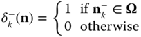
When ![]() , the compressed bandwidth
, the compressed bandwidth ![]() of the newly accepted call of service‐class k, is given by [ 1]:
of the newly accepted call of service‐class k, is given by [ 1]:

where ![]() denotes the compression factor.
denotes the compression factor.
Since ![]() , where
, where ![]() is the number of in‐service calls of service‐class k (in the steady state),
is the number of in‐service calls of service‐class k (in the steady state), ![]() and
and ![]() , the values of
, the values of ![]() can be expressed by:
can be expressed by:

To keep constant the product service time by bandwidth per call (when bandwidth compression occurs), the mean service time of the new service‐class ![]() call becomes
call becomes ![]() :
:

The compressed bandwidth of all in‐service calls changes to ![]() for
for ![]() and
and ![]() . Similarly, their remaining service time increases by a factor of
. Similarly, their remaining service time increases by a factor of ![]() . The minimum bandwidth given to a service‐class
. The minimum bandwidth given to a service‐class ![]() call is:
call is:
where ![]() and is common for all service‐classes.
and is common for all service‐classes.
Note that increasing T decreases the ![]() and increases the delay (service‐time) of service‐class
and increases the delay (service‐time) of service‐class ![]() calls (compared to the initial service time
calls (compared to the initial service time ![]() ). Thus, T should be chosen so that this delay remains within acceptable levels.
). Thus, T should be chosen so that this delay remains within acceptable levels.
When an in‐service call, with compressed bandwidth ![]() , completes its service and departs from the system, then the remaining in‐service calls expand their bandwidth to
, completes its service and departs from the system, then the remaining in‐service calls expand their bandwidth to ![]() in proportion to
in proportion to ![]() , as follows:
, as follows:

In terms of the system's state‐space ![]() , the CAC is expressed as follows. A new call of service‐class k is accepted in the system if the system is in state
, the CAC is expressed as follows. A new call of service‐class k is accepted in the system if the system is in state ![]() upon a new call arrival, where
upon a new call arrival, where ![]() . Hence, the CBP of service‐class
. Hence, the CBP of service‐class ![]() is determined by the state space
is determined by the state space ![]() :
:

Unfortunately, the compression/expansion of bandwidth destroys the LB between adjacent states in the E‐EMLM, or, equivalently, it destroys the reversibility of the system's Markov chain, and therefore no PFS exists for the values of ![]() (a fact that makes 3.6 inefficient). To show that the Markov chain of the E‐EMLM is not reversible, an efficient way is to apply the so called Kolmogorov's criterion [3,4]: A Markov chain is reversible if and only if the product of transition probabilities along any loop of adjacent states is the same as that for the reversed loop.1
(a fact that makes 3.6 inefficient). To show that the Markov chain of the E‐EMLM is not reversible, an efficient way is to apply the so called Kolmogorov's criterion [3,4]: A Markov chain is reversible if and only if the product of transition probabilities along any loop of adjacent states is the same as that for the reversed loop.1
To circumvent the non‐reversibility problem in the E‐EMLM, ![]() are replaced by the state‐dependent compression factors per service‐class
are replaced by the state‐dependent compression factors per service‐class ![]() , which not only have a similar role with
, which not only have a similar role with ![]() but also lead to a reversible Markov chain [5]. Thus, (3.1) becomes:
but also lead to a reversible Markov chain [5]. Thus, (3.1) becomes:
Reversibility facilitates the recursive calculation of the link occupancy distribution (see Section 3.1.2). To ensure reversibility, ![]() must have the form [ 5]:
must have the form [ 5]:

where ![]() and
and ![]() .
.
In (3.8), ![]() is a state multiplier associated with state
is a state multiplier associated with state ![]() , whose values are chosen so that
, whose values are chosen so that ![]() holds whenever
holds whenever ![]() , that is,
, that is, ![]() is given by [ 5]:
is given by [ 5]:

3.1.2 The Analytical Model
3.1.2.1 Steady State Probabilities
The steady state transition rates of the E‐EMLM are shown in Figure 3.4. According to this, the GB equation (rate in = rate out) for state ![]() is given by:
is given by:

where ![]()
 ,
,  , and
, and ![]() are the probability distributions of the corresponding states
are the probability distributions of the corresponding states ![]() , respectively.
, respectively.

Figure 3.4 State transition diagram of the E‐EMLM.
Assume now the existence of LB between adjacent states. Equations (3.11) and (3.12) are the detailed LB equations which exist because the Markov chain of the modified model is reversible. Then, based on Figure 3.4, the following LB equations are extracted:
for ![]() and
and ![]() .
.
Based on the LB assumption, the probability distribution ![]() has the solution:2
has the solution:2

where ![]() is the offered traffic‐load in erl and
is the offered traffic‐load in erl and ![]() is the normalization constant given by:
is the normalization constant given by:

Note that although the Markov chain has become reversible, the probability distribution ![]() of (3.13) is not a PFS due to the summation of (3.9) needed for the determination of
of (3.13) is not a PFS due to the summation of (3.9) needed for the determination of ![]() . We proceed by defining
. We proceed by defining ![]() , as:
, as:

where ![]() is the set of states in which exactly
is the set of states in which exactly ![]() b.u. are occupied by all in‐service calls, i.e.,
b.u. are occupied by all in‐service calls, i.e., ![]() .
.
Consider now two different sets of macro‐states: (i) ![]() and (ii)
and (ii) ![]() . For the first set, no bandwidth compression takes place and the values of
. For the first set, no bandwidth compression takes place and the values of ![]() are determined by the classical Kaufman–Roberts recursion (1.39). For the second set, aiming at deriving a similar recursion, we first substitute ( 3.8) in ( 3.11) to obtain:
are determined by the classical Kaufman–Roberts recursion (1.39). For the second set, aiming at deriving a similar recursion, we first substitute ( 3.8) in ( 3.11) to obtain:
Multiplying both sides of (3.16) by ![]() and summing over k, we have:
and summing over k, we have:

Equation (3.17), due to ( 3.9) is written as:

Summing both sides of (3.18) over ![]() and based on (3.15), we have:
and based on (3.15), we have:

or

The combination of (1.39) and (3.20) results in the recursive formula of the E‐EMLM [ 5]:

3.1.2.2 CBP, Utilization, and Mean Number of In‐service Calls
The following performance measures can be determined based on (3.21):
- The CBP of service‐class k,
 , via:
(3.22)where
, via:
(3.22)where
 is the normalization constant.
 - The link utilization,
 , via:
(3.23)
, via:
(3.23)
- The average number of service‐class k calls in the system,
 , via:
(3.24)where
, via:
(3.24)where
 is the average number of service‐class
  calls given that the system (macro‐)state is
  , and is determined by [6]:
(3.25)where
, and is determined by [6]:
(3.25)where
 , while
  for
for  and
and  .
.
3.1.2.3 Relationship between the E‐EMLM and the Balanced Fair Share Model
In the literature, a similar model exists called the balanced fair share model [7,8], which aims to share the capacity of a single link among elastic calls already accepted for service according to a balanced fairness criterion, whereas the E‐EMLM focuses on call admission. In what follows, we show that the bandwidth compression mechanism of the E‐EMLM and the model of [ 7, 8] provide the same bandwidth compression.
In [ 8], a link accommodates Poisson arriving calls of ![]() elastic service‐classes. The link capacity
elastic service‐classes. The link capacity ![]() is shared among calls according to the balanced fairness criterion: when
is shared among calls according to the balanced fairness criterion: when ![]() , all calls use their peak‐bandwidth requirement, while when
, all calls use their peak‐bandwidth requirement, while when ![]() , all calls share the capacity
, all calls share the capacity ![]() in proportion to their peak‐bandwidth requirement and the link operates at its full capacity
in proportion to their peak‐bandwidth requirement and the link operates at its full capacity ![]() . The main difference between the E‐EMLM and the model of [ 8] lies on the fact that in the E‐EMLM, the notion of
. The main difference between the E‐EMLM and the model of [ 8] lies on the fact that in the E‐EMLM, the notion of ![]() allows for admission control, whereas there is no such parameter in [ 8]. The application of balanced fairness in multirate networks and its comparison with other classical bandwidth allocation policies, such as max–min fairness and proportional fairness can be found in [9,10]. See Example 3.11 for a comparison between the approach of [ 9] and the compression mechanism of the E‐EMLM under a threshold policy.
allows for admission control, whereas there is no such parameter in [ 8]. The application of balanced fairness in multirate networks and its comparison with other classical bandwidth allocation policies, such as max–min fairness and proportional fairness can be found in [9,10]. See Example 3.11 for a comparison between the approach of [ 9] and the compression mechanism of the E‐EMLM under a threshold policy.
According to [ 8], the balanced fair sharing ![]() of all
of all ![]() calls of service‐class
calls of service‐class ![]() in state
in state ![]() is given by:
is given by:

where ![]() is a balance function defined by:
is a balance function defined by:

and ![]() is the unit line vector with 1 in the
is the unit line vector with 1 in the ![]() element and 0 elsewhere. According to (3.27), when
element and 0 elsewhere. According to (3.27), when ![]() , (3.26) is written as [ 8]:
, (3.26) is written as [ 8]:

The balance fair share model determines (through (3.28)) the total bandwidth which will be allocated to each service‐class, whereas the E‐EMLM determines (through ( 3.8)) the percentage of the peak‐bandwidth per call requirement which will be assigned to each call of each service‐class. This percentage has a limit which is defined through the ![]() parameter, while the absence of
parameter, while the absence of ![]() in the balance fair share model means that there is no limitation in bandwidth compression. The relationship between the
in the balance fair share model means that there is no limitation in bandwidth compression. The relationship between the ![]() of the E‐EMLM and the
of the E‐EMLM and the ![]() of the balance fair share model is
of the balance fair share model is ![]() . To show this, let
. To show this, let ![]() service‐classes (for presentation purposes). Assuming that in state
service‐classes (for presentation purposes). Assuming that in state ![]() , i.e.,
, i.e., ![]() or
or ![]() , calls of service‐class
, calls of service‐class ![]() use their peak‐bandwidth requirements, the balanced fairness allocation gives:
use their peak‐bandwidth requirements, the balanced fairness allocation gives:

Similarly,

So, in state ![]() , where C
, where C ![]() nb, the bandwidth allocated to a service‐class k call is:
nb, the bandwidth allocated to a service‐class k call is:

Based on ( 3.8) and ( 3.9), the E‐EMLM gives:

assuming that ![]() (i.e., no bandwidth compression takes place in state
(i.e., no bandwidth compression takes place in state ![]() ). Combining (3.31) with (3.32), we obtain
). Combining (3.31) with (3.32), we obtain ![]() .
.
3.2 The Elastic Erlang Multirate Loss Model under the BR Policy
3.2.1 The Service System
We now consider the multiservice system of the E‐EMLM under the BR policy (E‐EMLM/ BR): A new service‐class ![]() call is accepted in the link, if after its acceptance, the occupied link bandwidth
call is accepted in the link, if after its acceptance, the occupied link bandwidth ![]() , where
, where ![]() refers to the BR parameter used to benefit (in CBP) calls of other service‐classes apart from
refers to the BR parameter used to benefit (in CBP) calls of other service‐classes apart from ![]() (see also the EMLM/BR in Section 1.3.2).
(see also the EMLM/BR in Section 1.3.2).
In terms of the system state‐space ![]() , the CAC is expressed as follows. A new call of service‐class
, the CAC is expressed as follows. A new call of service‐class ![]() is accepted in the system if the system is in state
is accepted in the system if the system is in state ![]() upon a new call arrival, where
upon a new call arrival, where ![]() . Hence, the CBP of service‐class
. Hence, the CBP of service‐class ![]() is determined by the state space
is determined by the state space ![]() :
:

As far as the compression factors and the state dependent compression factors per service‐class are concerned, they are determined by (3.2) and ( 3.8), respectively.
3.2.2 The Analytical Model
3.2.2.1 Link Occupancy Distribution
In the E‐EMLM/BR, the link occupancy distribution, ![]() , can be calculated in an approximate way, according to the Roberts method (see Section 1.3.2.2), which leads to the following recursive formula [11]:
, can be calculated in an approximate way, according to the Roberts method (see Section 1.3.2.2), which leads to the following recursive formula [11]:

This formula is similar to (1.64) of the EMLM/BR. If ![]() for all
for all ![]() then the E‐EMLM results. In addition, if
then the E‐EMLM results. In addition, if ![]() then we have the classical EMLM.
then we have the classical EMLM.
3.2.2.2 CBP, Utilization, and Mean Number of In‐service Calls
The following performance measures can be determined based on (3.34):

3.3 The Elastic Erlang Multirate Loss Model under the Threshold Policy
3.3.1 The Service System
We now consider the multi‐service system of the E‐EMLM under the TH policy (E‐EMLM/ TH), as follows. A new call of service‐class ![]() is accepted in the system, of
is accepted in the system, of ![]() b.u., if [12]:
b.u., if [12]:
- (i) The number of in‐service calls of service‐class
 , together with the new call, does not exceed a threshold
  , i.e.,
  . Otherwise the call is blocked. This constraint expresses the TH policy.
 - (ii) If constraint (i) is met, then: (a) If
 , the call is accepted in the system with
  b.u. and remains in the system for an exponentially distributed service time with mean
  . (b) If
  the call is accepted by compressing its
  together with the bandwidth of all in‐service calls of all service‐classes. The bandwidth compression/expansion mechanism is identical to the one described in Section 3.1.
In terms of the system state‐space ![]() , the CAC is expressed as follows. A new call of service‐class
, the CAC is expressed as follows. A new call of service‐class ![]() is accepted in the system if the system is in state
is accepted in the system if the system is in state ![]() upon a new call arrival, where
upon a new call arrival, where ![]() . Hence, the CBP of service‐class
. Hence, the CBP of service‐class ![]() is determined by the state space
is determined by the state space ![]() :
:

3.3.2 The Analytical Model
3.3.2.1 Steady State Probabilities
The steady state transition rates of the E‐EMLM/TH are shown in Figure 3.4. According to this, the GB equation for state ![]() is given by (3.10), while the LB equations are given by ( 3.11) and ( 3.12) where:
is given by (3.10), while the LB equations are given by ( 3.11) and ( 3.12) where: ![]() .
.
Based on the LB assumption, the probability distribution ![]() has the solution of ( 3.13) where the normalization constant is given by (3.14). Since
has the solution of ( 3.13) where the normalization constant is given by (3.14). Since ![]() is the occupied link bandwidth, we consider two different sets of macro‐states: (i)
is the occupied link bandwidth, we consider two different sets of macro‐states: (i) ![]() and (ii)
and (ii) ![]() . For set (i), no bandwidth compression takes place and
. For set (i), no bandwidth compression takes place and ![]() are determined via (1.73). For set (ii), we follow the analysis of the E‐EMLM up to (3.19). Since
are determined via (1.73). For set (ii), we follow the analysis of the E‐EMLM up to (3.19). Since ![]() , we have:
, we have:

Thus, ( 3.19) can be written as:

where ![]() is the probability that
is the probability that ![]() b.u. are occupied when the number of service‐class
b.u. are occupied when the number of service‐class ![]() in‐service calls is
in‐service calls is ![]() , and is determined by (1.74). The combination of (1.73) and (3.38) results in the recursive formula of the E‐EMLM/TH [ 12]:
, and is determined by (1.74). The combination of (1.73) and (3.38) results in the recursive formula of the E‐EMLM/TH [ 12]:

3.3.2.2 CBP, Utilization, and Mean Number of In‐service Calls
The following performance measures can be determined based on (3.39):
- The CBP of service‐class
 ,
,  , via:
(3.40)where
, via:
(3.40)where
 is the normalization constant.
 - The link utilization,
 , according to ( 3.23).
 - The average number of service‐class
 calls in the system,
  , via:
(3.41)where
, via:
(3.41)where
 is the average number of service‐class
  calls given that the system state is
  , and is given by:
(3.42)where
, and is given by:
(3.42)where
 , while
  for
for  and
and  .
.
In ( 3.39), knowledge of ![]() is required. Since
is required. Since ![]() when
when ![]()
![]() , we distinguish two regions of
, we distinguish two regions of ![]() : (i)
: (i) ![]() and (ii)
and (ii) ![]() .
.
For the first region (where no bandwidth compression occurs), consider a system of capacity ![]() that accommodates all service‐classes but service‐class
that accommodates all service‐classes but service‐class ![]() . For this system, we define
. For this system, we define ![]() as follows:
as follows:

Based on ![]() , we compute the unnormalized
, we compute the unnormalized ![]() , recursively, via the following formula:
, recursively, via the following formula:

For the second region (where bandwidth compression occurs), the values of ![]() can be determined (taking into account ( 3.9)) by:
can be determined (taking into account ( 3.9)) by:

where ![]() .
.
3.4 The Elastic Adaptive Erlang Multirate Loss Model
3.4.1 The Service System
In the elastic adaptive EMLM (EA‐EMLM), we consider a link of capacity ![]() b.u. that accommodates
b.u. that accommodates ![]() service‐classes which are distinguished into
service‐classes which are distinguished into ![]() elastic service‐classes and
elastic service‐classes and ![]() adaptive service‐classes,
adaptive service‐classes, ![]() . The call arrival process remains Poisson. As already mentioned, adaptive traffic is considered a variant of elastic traffic in the sense that adaptive calls can tolerate bandwidth compression without altering their service time.
. The call arrival process remains Poisson. As already mentioned, adaptive traffic is considered a variant of elastic traffic in the sense that adaptive calls can tolerate bandwidth compression without altering their service time.
The bandwidth compression/expansion mechanism and the CAC of the EA‐EMLM are the same as those of the E‐EMLM (Section 3.1.1). The only difference is in (3.3), which is applied only on elastic calls. Similar to the E‐EMLM, the corresponding Markov chain in the EA‐EMLM does not meet the necessary and sufficient Kolmogorov's criterion for reversibility between four adjacent states.
To circumvent the non‐reversibility problem in the EA‐EMLM, similar to the E‐EMLM, ![]() are replaced by the state‐dependent factors per service‐class
are replaced by the state‐dependent factors per service‐class ![]() ,
, ![]() , which individualize the role of
, which individualize the role of ![]() per service‐class in order to lead to a reversible Markov chain [6]. Thus the compressed bandwidth of service‐class
per service‐class in order to lead to a reversible Markov chain [6]. Thus the compressed bandwidth of service‐class ![]() calls is determined by (3.7), while the values of
calls is determined by (3.7), while the values of ![]() are given by ( 3.8). However, due to the adaptive service‐classes, in the EA‐EMLM the values of the state multipliers
are given by ( 3.8). However, due to the adaptive service‐classes, in the EA‐EMLM the values of the state multipliers ![]() are determined by [ 6]:
are determined by [ 6]:

where ![]() .
.
The derivation of (3.47) is based on the following assumptions:
- (i) The bandwidth of all in‐service calls of service‐class
 (elastic or adaptive) is compressed by a factor
  to a new value
  in state
  , where
  , so that:
(3.48)
, so that:
(3.48)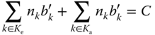
- (ii) The product service time by bandwidth per call of service‐class
 calls,
  , remains the same in state
  regardless of the reversibility of the Markov chain. In other words, it holds that:
(3.49)
regardless of the reversibility of the Markov chain. In other words, it holds that:
(3.49) (3.50)
Now, we can derive ( 3.47) by substituting (3.49), 3.50, and 3.8 into 3.48.
3.4.2 The Analytical Model
3.4.2.1 Steady State Probabilities
The steady state transition rates of the EA‐EMLM are shown in Figure 3.4. According to this, the GB equation for state ![]() is given by ( 3.10) and the LB equations by ( 3.11) and ( 3.12).
is given by ( 3.10) and the LB equations by ( 3.11) and ( 3.12).
Similar to the E‐EMLM, we consider two different sets of macro‐states: (i) ![]() and (ii)
and (ii) ![]() . For set (i), no bandwidth compression takes place and
. For set (i), no bandwidth compression takes place and ![]() are determined by the classical Kaufman–Roberts recursion (1.39). For set (ii), we substitute ( 3.8) in ( 3.11) to have:
are determined by the classical Kaufman–Roberts recursion (1.39). For set (ii), we substitute ( 3.8) in ( 3.11) to have:
Multiplying both sides of (3.51a) by ![]() and summing over
and summing over ![]() , we take:
, we take:

Similarly, multiplying both sides of (3.51b) by ![]() and
and ![]() , and summing over
, and summing over ![]() , we take:
, we take:

By adding (3.52) and (3.53), we have:

Based on ( 3.47), (3.54) is written as:

Summing both sides of (3.55) over ![]() and based on the fact that
and based on the fact that ![]() , we have:
, we have:

The combination of (1.39) and (3.56) leads to the recursive formula of the EA‐EMLM [ 6]:

3.4.2.2 CBP, Utilization, and Mean Number of In‐service Calls
The following performance measures can be determined based on (3.57):


3.5 The Elastic Adaptive Erlang Multirate Loss Model under the BR Policy
3.5.1 The Service System
We now consider the multiservice system of the EA‐EMLM under the BR policy (EA‐EMLM/BR) [13]. A new service‐class ![]() call is accepted in the link if, after its acceptance, the occupied link bandwidth
call is accepted in the link if, after its acceptance, the occupied link bandwidth ![]() , where
, where ![]() refers to the BR parameter used to benefit (in CBP) calls of other service‐classes apart from
refers to the BR parameter used to benefit (in CBP) calls of other service‐classes apart from ![]() . In terms of the system state‐space
. In terms of the system state‐space ![]() , the CBP is expressed according to ( 3.33).
, the CBP is expressed according to ( 3.33).
3.5.2 The Analytical Model
3.5.2.1 Link Occupancy Distribution
In the EA‐EMLM/BR, the link occupancy distribution, ![]() , is calculated in an approximate way, according to the following recursive formula (Roberts method) [ 13]:
, is calculated in an approximate way, according to the following recursive formula (Roberts method) [ 13]:


This formula is similar to (3.34) of the E‐EMLM/BR. If ![]() for all
for all ![]() , then the EA‐EMLM results. In addition, if
, then the EA‐EMLM results. In addition, if ![]() , then we have the classical EMLM.
, then we have the classical EMLM.
3.5.2.2 CBP, Utilization, and Mean Number of In‐service Calls
The following performance measures can be determined via (3.60):
- The CBP of service‐class
 , via ( 3.35).
 - The link utilization,
 , via ( 3.23).
 - The average number of service‐class
 calls in the system,
  , is determined by ( 3.24), where
  are given by ( 3.58) and ( 3.59) for elastic and adaptive service‐classes, respectively, under the assumptions that (i)
  when
when  and (ii)
  when
when  .
.
3.6 The Elastic Adaptive Erlang Multirate Loss Model under the Threshold Policy
3.6.1 The Service System
We now consider the EA‐EMLM under the TH policy (EA‐EMLM/TH), as in the case of the E‐EMLM/TH (Section 3.3). That is, the total number of in‐service calls per service‐class must not exceed a threshold (per service‐class). The bandwidth compression/expansion mechanism and the CAC in the EA‐EMLM/TH are the same as those of the E‐EMLM/TH, but ( 3.3) is applied only on elastic calls to satisfy their service time requirement.
3.6.2 The Analytical Model
3.6.2.1 Steady State Probabilities
The steady state transition rates of the EA‐EMLM/TH are shown in Figure 3.4. According to this, the GB equation for state ![]()
![]() is given by ( 3.10), while the LB equations are given by ( 3.11) and ( 3.12) where
is given by ( 3.10), while the LB equations are given by ( 3.11) and ( 3.12) where ![]() .
.
Similar to the EA‐EMLM, we consider two different sets of macro‐states: (i) ![]() and (ii)
and (ii) ![]() . For set (i), no bandwidth compression takes place and
. For set (i), no bandwidth compression takes place and ![]() are determined via (1.73). For set (ii), in order to derive a recursive formula, we follow the analysis of the EA‐EMLM up to ( 3.55). Since
are determined via (1.73). For set (ii), in order to derive a recursive formula, we follow the analysis of the EA‐EMLM up to ( 3.55). Since ![]() , we have:
, we have:

Thus, ( 3.55) can be written as:

where ![]() expresses the blocking constraint of the TH policy and is given by (1.74).
expresses the blocking constraint of the TH policy and is given by (1.74).
Summing both sides of (3.62) over ![]() and based on the fact that
and based on the fact that ![]() , we have:
, we have:

The combination of (1.73) and (3.63) results in the formula of the EA‐EMLM/TH [14]:

3.6.2.2 CBP, Utilization, and Mean Number of In‐service Calls
The following performance measures can be determined based on (3.64):
- The CBP of service‐class
 , via ( 3.40).
 - The link utilization,
 , according to ( 3.23).
 - The average number of service‐class
 calls in the system,
  , via ( 3.24) where the values of
  are given by (3.65) for elastic traffic and (3.66) for adaptive traffic:
(3.65)
are given by (3.65) for elastic traffic and (3.66) for adaptive traffic:
(3.65) (3.66)where
 , while
  for
for  and
and  .
.
In ( 3.64) knowledge of ![]() is required. Since
is required. Since ![]() when
when ![]()
![]() , we consider two subsets of
, we consider two subsets of ![]() : (i)
: (i) ![]() and (ii)
and (ii) ![]() . In both subsets, we assume that
. In both subsets, we assume that ![]() .
.
For the first subset, let a system of capacity ![]() that accommodates all service‐classes but service‐class
that accommodates all service‐classes but service‐class ![]() . For this system, we define
. For this system, we define ![]() via (3.43). Based on
via (3.43). Based on ![]() , we compute
, we compute ![]() through (3.44). For the second subset,
through (3.44). For the second subset, ![]() can be determined via (3.45).
can be determined via (3.45).
3.7 Applications
We discuss the applicability of the models in the context of new architectural and functional enhancements of next‐generation (5G) cellular networks. It is widely acknowledged that 5G systems will extensively rely on software‐defined networking (SDN) and network function virtualization (NFV), which have attracted a lot of research efforts and gained tremendous attention from both academic and industry communities. The SDN technology is the driver towards completely programmable networks, which can be achieved by decoupling the control and data planes [15,16]. On the other hand, the NFV technology allows executing the software‐based network functions on general‐purpose hardware via virtualization [17,18]. SDN and NFV, due to their complementary nature, are traditionally seen as related concepts and implemented together [19]. Some of the expected benefits of SDN/NFV include CAPEX and OPEX reduction for network operators, by reducing the cost of hardware and automating services, flexibility in terms of deployment and operation of new infrastructure and applications, faster innovation cycles due to the creation of enhanced services/applications, and new business models. Due to these benefits, SDN/NFV will play a major role in the emerging 5G systems [20]. In what follows, we briefly describe the considered SDN/NFV based cellular network architecture, shown in Figure 3.32, and its main elements [21].

Figure 3.32 SDN/NFV based next‐generation network architecture.
The realization of an intelligent radio access network (RAN) is greatly facilitated by SDN and NFV technologies [22]. SDN enables abstraction and modularity of the network functions at the RAN level. As a consequence, a hierarchical control architecture can be implemented, in which the high control layer controls lower layers by specifying procedures and without the requirement to have access to the specific implementation details of the lower layers [23]. Such an implementation, however, requires a holistic view of the cellular network at the higher control layer to be designed by taking into account appropriate abstraction of lower layers via well‐defined control interfaces. This is essential to enable programmable radio resource management (RRM) functions, such as radio resource allocation (RRA) and CAC. On the other hand, NFV technology allows the execution of control programs on general purpose computing/storage resources [24]. This is contrary to the traditional approach in which the BS consists of a tightly coupled software and hardware platforms. Hence, an NFV‐based BS may have some network functions implemented as physical network functions, while other functions are implemented as virtual network functions (VNFs). An advantage of VNFs is that the underlying hardware can be efficiently utilized since VNFs run on shared NFV infrastructure (NFVI).
The architecture of Figure 3.32 relies on the SDN concept, whose different layers are depicted in Figure 3.33. In the control layer, the SDN controller provides a global view of the available underlying resources to one or more network applications that are located at the application layer. This communication is done using the so‐called northbound open application programming interface (API). On the other hand, the southbound open API is used to configure the forwarding elements (FEs) that are located at the infrastructure layer. The configuration of FEs is performed by the SDN controller, which sends control messages to the SDN agents located within the FEs.

Figure 3.33 Layering concept in SDN.
The main elements at the RAN level are small cell BSs (SBSs), macro BSs (MBSs), WiFi APs, local offload gateways (LO‐GWs) [25], and mobile users (MUs). These entities are controlled by the local SDN controller (LSC). The geographical area of the RAN consists of a number of clusters. Each cluster typically consists of many cells and is under the control of a single LSC. For example, in Figure 3.32 the first cluster contains one MBS, one SBS, one WiFi AP, one LO‐GW, and four MUs, whereas the second cluster contains one MBS and three MUs. MUs can freely move between clusters or even may belong to more than one cluster at the same time.
When a network entity wishes to establish a connection, it sends the request to the corresponding LSC of the cluster. Upon receiving the request, the LSC will identify the appropriate destination address for the requested connection. In particular, the LSC will forward the request to either the appropriate in‐cluster recipient (e.g. MU or MBS) or the mobile core network (MCN) if the recipient is outside the cluster. To be able to perform this, the LSC maintains the knowledge of the cluster topology as well as the external connections towards the MCN and neighbouring clusters. The LSC is also responsible for multi radio access technologies (RATs) coordination, that is, it takes the RRA decisions in geographical areas where multiple RATs are available (e.g., LTE and WiFi). In the cache‐enabled mode [26], the LSC takes caching decisions within the cluster by exploiting the knowledge of content popularity and available in‐cluster resources. Another important function of the LSC is in‐cluster content routing. Upon receiving the connection request from an MU, the LSC constructs the path from the content source (if the source is within the cluster) or the border entity (if the source is outside the cluster) towards the requesting MU. The LSC then modifies the flow tables at the FEs along the content delivery path. Finally, the LCS is responsible for MU mobility within its cluster. Hence, mobility‐related information does not need to be sent over to the MCN. In Figure 3.34, the basic components of a virtualized RAN are shown. Multiple virtual BSs (VBSs) may run on top of the NFVI, essentially sharing the resources of the same physical infrastructure.

Figure 3.34 SDN/NFV based RAN.
The MCN consists of the mobile cloud computing (MCC) infrastructure, mobile content delivery network (M‐CDN) servers, packet data network (PDN) GWs and serving GWs (S‐GWs). The control is performed by one or more core SDN controllers (CSCs). A CSC receives and handles the connection requests from the RAN via the corresponding LSCs. A CSC is also responsible for storage (e.g., M‐CDN), compute (e.g., MCC), spectrum, and energy resources, and for providing QoS support. Finally, the PDN‐GW (or simply P‐GW) forwards traffic to/from the Internet and other external IP networks, whereas the S‐GW receives/sends traffic from/to the RAN.
We continue by describing our considered RAN model in the SDN/NFV‐enabled cellular network [ 21]. We assume a cluster of VBSs controlled by a single LSC at the RAN level (Figure 3.34). The cluster has a fixed number ![]() of VBSs. For the purposes of the analysis it is assumed that the amount of radio resources in the RAN can be discretized and is measured in resource units (RUs). The RU definition depends on the adopted channel access scheme. When schemes based on the FDMA and the TDMA are used, the RU can be defined as an integer number of frequency carriers or time slots. On the other hand, when schemes based on the CDMA are used, the definition of the RU must take into account the multiple access interference [27]. To this end, the notions of the cell load and load factor have been used [28,29]. In [ 21], the LTE orthogonal FDMA (OFDMA) scheme is adopted. We define a RU to be equal to a single OFDMA resource block (RB). For example, if the LTE channel bandwidth is 9 MHz and one subcarrier is 15 kHz, then there are in total 600 subcarriers. Since one OFDMA RB corresponds to 12 subcarriers, we have 50 RUs per channel per time slot. Similarly, a 13.5 MHz LTE channel has 75 RUs and a 18 MHz LTE channel has 100 RUs.
of VBSs. For the purposes of the analysis it is assumed that the amount of radio resources in the RAN can be discretized and is measured in resource units (RUs). The RU definition depends on the adopted channel access scheme. When schemes based on the FDMA and the TDMA are used, the RU can be defined as an integer number of frequency carriers or time slots. On the other hand, when schemes based on the CDMA are used, the definition of the RU must take into account the multiple access interference [27]. To this end, the notions of the cell load and load factor have been used [28,29]. In [ 21], the LTE orthogonal FDMA (OFDMA) scheme is adopted. We define a RU to be equal to a single OFDMA resource block (RB). For example, if the LTE channel bandwidth is 9 MHz and one subcarrier is 15 kHz, then there are in total 600 subcarriers. Since one OFDMA RB corresponds to 12 subcarriers, we have 50 RUs per channel per time slot. Similarly, a 13.5 MHz LTE channel has 75 RUs and a 18 MHz LTE channel has 100 RUs.
Let us denote by ![]() the total number of RUs in the RAN. RUs are dynamically allocated by the LSC to the VBSs such that the VBS
the total number of RUs in the RAN. RUs are dynamically allocated by the LSC to the VBSs such that the VBS ![]() receives
receives ![]() RUs. Hence, at any given moment it must hold that:
RUs. Hence, at any given moment it must hold that:

Considering ![]() different service‐classes, they are distinguished by the number of RUs requested by a single call that originates from a MU. We assume that the calls follow a Poisson distribution. The arrival rate of service‐class
different service‐classes, they are distinguished by the number of RUs requested by a single call that originates from a MU. We assume that the calls follow a Poisson distribution. The arrival rate of service‐class ![]() calls is denoted as
calls is denoted as ![]() . A service‐class
. A service‐class ![]() call requests
call requests ![]() RUs. Let
RUs. Let ![]() be the occupied RUs in the cluster and assume that
be the occupied RUs in the cluster and assume that ![]() can virtually exceed
can virtually exceed ![]() up to a limit of
up to a limit of ![]() RUs. Then the CAC of a service‐class
RUs. Then the CAC of a service‐class ![]() call may follow the one described in Section 3.1.1 for the E‐EMLM.
call may follow the one described in Section 3.1.1 for the E‐EMLM.
We showed the method of applying the E‐EMLM in next‐generation networks. It is worth mentioning that almost all teletraffic models can be applied in the same manner, after some necessary adjustments.
3.8 Further Reading
An interesting extension of the E‐EMLM includes the co‐existence of stream and elastic traffic with or without prioritization of stream traffic [30–32]. In both cases there is no single recursive formula for the calculation of the link occupancy distribution. In the case of stream traffic prioritization, the CBP calculation of stream (not elastic) calls can be based on the Kaufman–Roberts formula. On the other hand, in the case of no prioritization, the CBP determination of stream and elastic calls can only be based on approximate (non‐recursive) algorithms [ 32]. An interesting extension of the E‐EMLM is proposed in [33], in which the E‐EMLM is described as a multirate loss‐queueing model with a finite number of buffers, a fact that provides a springboard for the efficient analysis of multirate queues. A generalization of [ 33] that provides a framework for the calculation of various queueing characteristics for each elastic service‐class is proposed in [34]. The case of adaptive traffic is studied in [35].
Another interesting model (since it is recursive) for elastic traffic in wireless networks has been proposed in [36], where the uplink of a CDMA cell is analysed. Service‐class ![]() calls arrive following a Poisson process with rate
calls arrive following a Poisson process with rate ![]() and having a peak transmission bit rate requirement,
and having a peak transmission bit rate requirement, ![]() . The service time is exponentially distributed with mean
. The service time is exponentially distributed with mean ![]() . When sending with the peak bit rate, the required target ratio of the received power from the mobile terminal to the total interference energy at the BS is given by [ 36]:
. When sending with the peak bit rate, the required target ratio of the received power from the mobile terminal to the total interference energy at the BS is given by [ 36]:
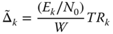
where ![]() is the bit‐energy‐to‐noise ratio and
is the bit‐energy‐to‐noise ratio and ![]() is the spread spectrum bandwidth.
is the spread spectrum bandwidth.
Let ![]() be the number of in‐service service‐class
be the number of in‐service service‐class ![]() calls and
calls and ![]() the power received at the BS from the user equipment (UE). The power
the power received at the BS from the user equipment (UE). The power ![]() should fulfil the equation [ 36]:
should fulfil the equation [ 36]:

where ![]() is the total power received by the BS within its cell,
is the total power received by the BS within its cell, ![]() is the total power received from other cells and
is the total power received from other cells and ![]() is the background noise power.
is the background noise power.
Based on (3.68) we obtain the following equation for ![]() [ 36]:
[ 36]:

According to the denominator of (3.69), we see that the CAC must prevent ![]() becoming larger than
becoming larger than ![]() .
.
Finally, it can be proved (see [ 36,37]) that there exists a recursive formula for the determination of CBP in a CDMA cell of maximum capacity ![]() which accommodates Poisson arriving calls of
which accommodates Poisson arriving calls of ![]() different service‐classes with offered traffic‐load
different service‐classes with offered traffic‐load ![]() and bandwidth requirement
and bandwidth requirement ![]() .
.
References
- 1 G. Stamatelos and V. Koukoulidis, Reservation‐based bandwidth allocation in a radio ATM network. IEEE/ACM Transactions on Networking, 5(3):420–428, June 1997.
- 2 S. Yashkov and A. Yashkova, Processor sharing: A survey of the mathematical theory. Automation and Remote Control, 68(9):1662–1731, September 2007.
- 3 R. Dobrushin, Yu. Sukhov and J. Fritz, A.N. Kolmogorov – the founder of the theory of reversible Markov processes. Russian Mathematical Surveys, 43(6):157–182, 1988.
- 4 V. Iversen, Reversible fair scheduling: The teletraffic theory revisited. Proceedings of the 20th International Teletraffic Congress, LNCS 4516, pp. 1135–1148, Ottawa, Canada, June 2007.
- 5 V. Koukoulidis, A characterization of reversible Markov processes with applications to shared‐resource environments, PhD thesis, Concordia University, Montreal, Canada, April 1993.
- 6 S. Racz, B. Gero and G. Fodor, Flow level performance analysis of a multi‐service system supporting elastic and adaptive services. Performance Evaluation, 49(1–4): 451–469, September 2002.
- 7 T. Bonald, A. Proutiere, J. Roberts and J. Virtamo, Computational aspects of balanced fairness. Proceedings of the International Teletraffic Congress (ITC) 18, Berlin, Germany, September 2003.
- 8 T. Bonald and J. Virtamo, A recursive formula for multirate systems with elastic traffic. IEEE Communications Letters, 9(8):753–755, August 2005.
- 9 T. Bonald and J. Virtamo, Calculating the flow level performance of balanced fairness in tree networks. Performance Evaluation, 58(1):1–14, October 2004.
- 10 T. Bonald, L. Massoulie, A. Proutiere and J. Virtamo, A queueing analysis of max‐min fairness, proportional fairness and balanced fairness. Queueing Systems, 53(1): 65–84, June 2006.
- 11 I. Moscholios, V. Vassilakis, M. Logothetis and A. Boucouvalas, Blocking equalization in the Erlang multirate loss model for elastic traffic. Proceedings of the 2nd International Conference on Emerging Network Intelligence (EMERGING), Florence, Italy, October 2010.
- 12 I. Moscholios, M. Logothetis, A. Boucouvalas and V. Vassilakis, An Erlang multirate loss model supporting elastic traffic under the threshold policy. Proceedings of the IEEE International Communications Conference (ICC), London, UK, June 2015.
- 13 I. Moscholios, V. Vassilakis, M. Logothetis and J. Vardakas, Bandwidth reservation in the Erlang multirate loss model for elastic and adaptive traffic. Proceedings of the 9th Advanced International Conference on Telecommunications (AICT), Rome, Italy, June 2013.
- 14 I. Moscholios, M. Logothetis and A. Boucouvalas, Blocking probabilities of elastic and adaptive calls in the Erlang multirate loss model under the threshold policy. Telecommunication Systems, 62(1): 245–262, May 2016.
- 15 B. Nunes, M. Mendonca, X. Nguyen, K. Obraczka and T. Turletti, A survey of software‐defined networking: past, present and future of programmable networks. IEEE Communications Surveys & Tutorials, 16(3): 1617–1634, third quarter 2014.
- 16 W. Xia, Y. Wen, C. Foh, D. Niyato and H. Xie, A survey on software‐defined networking. IEEE Communications Surveys & Tutorials, 17(1):27–51, first quarter 2015.
- 17 R. Mijumbi, J. Serrat, J. Gorricho, N. Bouten, F. Turck and R. Boutaba, Network function virtualization: state‐of‐the‐art and research challenges. IEEE Communications Surveys & Tutorials, 18(1):236–262, first quarter 2016.
- 18 B. Han, V. Gopalakrishnan, L. Ji and S. Lee, Network function virtualization: challenges and opportunities for innovations. IEEE Communications Magazine, 53(2):90–97, February 2015.
- 19 Q. Duan, N. Ansari and M. Toy, Software‐defined network virtualization: an architectural framework for integrating SDN and NFV for service provisioning in future networks. IEEE Network, 30(5):10–16, September–October 2016.
- 20 P. Agyapong, M. Iwamura, D. Staehle, W. Kiess and A. Benjebbour, Design considerations for a 5G network architecture. IEEE Communications Magazine, 52(11):65–75, November 2014.
- 21 V. Vassilakis, I. Moscholios and M. Logothetis, Efficient radio resource allocation in SDN/NFV based mobile cellular networks under the complete sharing policy. IET Networks, 7(3):103–108, May 2018.
- 22 V. Vassilakis, I. Moscholios, B. Alzahrani and M. Logothetis, A software‐defined architecture for next‐feneration cellular networks. Proceedings of the IEEE ICC, Kuala Lumpur, Malaysia, May 2016.
- 23 T. Chen, M. Matinmikko, X. Chen, X. Zhou and P. Ahokangas, Software defined mobile networks: concept, survey, and research directions. IEEE Communications Magazine, 53(11):126–133, November 2015.
- 24 F. Yousaf, M. Bredel, S. Schaller and F. Schneider, NFV and SDN key technology enablers for 5G networks. IEEE Journal on Selected Areas in Communications, 35(11):2468–2478, November 2017.
- 25 K. Samdanis, T. Taleb and S. Schmid, Traffic offload enhancements for eUTRAN. IEEE Communications Surveys & Tutorials, 14(3):884–896, third quarter 2012.
- 26 K. Poularakis, G. Iosifidis and L. Tassiulas, Approximation algorithms for mobile data caching in small cell networks. IEEE Transactions on Communications, 62(10):3665–3677, October 2014.
- 27 Y. Shen, Y. Wang, Z. Peng and S. Wu, Multiple‐access interference mitigation for acquisition of code‐division multiple access continuous‐wave signals. IEEE Communications Letters, 21(1):192–195, January 2017.
- 28 D. Staehle and A. Mäder, An analytic approximation of the uplink capacity in a UMTS network with heterogeneous traffic. Proceedings of the 18th International Teletraffic Congress (ITC18), Berlin, September 2003.
- 29 V. Vassilakis, I. Moscholios, A. Bontozoglou and M. Logothetis, Mobility‐aware QoS assurance in software – Defined radio access networks: An analytical study. Proceedings of the IEEE International Workshop on Software Defined 5G Networks, London, UK, April 2015.
- 30 M. Ivanovich and P. Fitzpatrick, An accurate performance approximation for beyond 3G wireless broadband systems with QoS. IEEE Transactions on Vehicular Technology, 62(5):2230–2238, June 2013.
- 31 Y. Huang, Z. Rosberg, K. Ko and M. Zukerman, Blocking probability approximations and bounds for best‐effort calls in an integrated service system. IEEE Transactions on Communications, 63(12):5014–5026, Dec. 2015.
- 32 B. Geró, P. Palyi, S. Rácz, Flow‐level performance analysis of a multi‐rate system supporting stream and elastic services. International Journal of Communication Systems, 26(8):974–988, August 2013.
- 33 S. Hanczewski, M. Stasiak and J. Weissenberg, A queueing model of a multi‐service system with state‐dependent distribution of resources for each class of calls. IEICE Transactions on Communications, E97‐B(8):1592–1605, August 2014.
- 34 M. Stasiak, Queuing systems for the Internet. IEICE Transactions on Communications, E99‐B(6):1234–1242, June 2016.
- 35 S. Hanczewski, M. Stasiak and J. Weissenberg, The model of the queuing system with adaptive traffic. Proceedings of the IEEE 19th International Conference on HPCC/Smart City/DSS, Bangkok, Thailand, December 2017.
- 36 G. Fodor and M. Telek, A recursive formula to calculate the steady state of CDMA networks. Proceedings of the ITC, Beijing, China, September 2005.
- 37 G. Fodor, Performance analysis of resource sharing policies in CDMA networks. International Journal of Communication Systems, 20(2):207–233, February 2007.