6
The Engset Multirate Loss Model
We start with quasi‐random arriving calls of fixed bandwidth requirements and fixed bandwidth allocation during service. Before the study of multirate teletraffic loss models, we begin with the simple case of a loss system that accommodates calls of a single service‐class.
6.1 The Engset Loss Model
6.1.1 The Service System
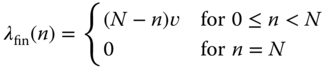
Consider a loss system of capacity ![]() b.u. which accommodates calls of a single service‐class. A call requires 1 b.u. to be connected in the system. If this bandwidth is available, then the call is accepted in the system and remains for an exponentially distributed service time, with mean value
b.u. which accommodates calls of a single service‐class. A call requires 1 b.u. to be connected in the system. If this bandwidth is available, then the call is accepted in the system and remains for an exponentially distributed service time, with mean value ![]() . Otherwise (when all b.u. are occupied), the call is blocked and lost without further affecting the system. What is important is that a call comes from a finite source population
. Otherwise (when all b.u. are occupied), the call is blocked and lost without further affecting the system. What is important is that a call comes from a finite source population ![]() , then the arrival process is smoother than the Poisson process and is known as quasi‐random [1]. The mean arrival rate of the idle sources is given by:
, then the arrival process is smoother than the Poisson process and is known as quasi‐random [1]. The mean arrival rate of the idle sources is given by:
where ![]() is the number of in‐service calls,
is the number of in‐service calls, ![]() is the number of idle sources in state
is the number of idle sources in state ![]() , while
, while ![]() is the arrival rate per idle source (constant).
is the arrival rate per idle source (constant).
6.1.2 The Analytical Model
6.1.2.1 Steady State Probabilities
We are interested in determining the steady state probability ![]() . To this end and similar to (1.4) we have the following steady state equation (which is the GB equation of state
. To this end and similar to (1.4) we have the following steady state equation (which is the GB equation of state ![]() ):
):
where ![]() and
and ![]() .
.
To determine ![]() , we solve (6.2) by applying the ladder method and hence we have:
, we solve (6.2) by applying the ladder method and hence we have:
which is the LB equation between the adjacent states ![]() and
and ![]() .
.
The graphical representation of ( 6.2) and (6.3) is given in Figure 6.1.

Figure 6.1 State transition diagram for the Engset loss model  .
.
From ( 6.3), by successive substitutions, we relate ![]() to the probability that the system is empty,
to the probability that the system is empty, ![]() :
:
where ![]() is the offered traffic‐load per idle source in erl.
is the offered traffic‐load per idle source in erl.
To determine ![]() , we know that:
, we know that:

That is,

By substituting (6.6) to (6.4), we determine ![]() :
:

which is known as the Engset distribution.
Assuming that ![]() and the total offered traffic‐load is constant (i.e.,
and the total offered traffic‐load is constant (i.e., ![]() ,
, ![]() ), then:
), then: ![]() , which means that the arrival process becomes Poisson, and (6.7) results in (1.9) (the Erlang distribution).
, which means that the arrival process becomes Poisson, and (6.7) results in (1.9) (the Erlang distribution).
As ![]() , the denominator of ( 6.7) becomes
, the denominator of ( 6.7) becomes ![]() and ( 6.7) is simplified to the binomial distribution:
and ( 6.7) is simplified to the binomial distribution:
where ![]() .
.
Since (1.9) and (6.8) can result from ( 6.7), one can consider ( 6.7) as a unified formula for the determination of the steady state probabilities in single rate loss systems.
6.1.2.2 CBP
To determine CBP in the Engset loss model, we initially need to derive a formula for the probability ![]() that
that ![]() calls exist in the system just prior to a new call arrival. Based on the Bayes and total probability theorems we have:
calls exist in the system just prior to a new call arrival. Based on the Bayes and total probability theorems we have:

Based on ( 6.4) and since ![]() , (6.9) is written as:
, (6.9) is written as:

By comparing (6.10) with ( 6.7) we see that:
The probabilities ![]() express how an internal observer perceives the system (as an internal observer we mean the call just accepted in the system), while the probabilities
express how an internal observer perceives the system (as an internal observer we mean the call just accepted in the system), while the probabilities ![]() express how an external observer perceives the system. According to (6.11),
express how an external observer perceives the system. According to (6.11), ![]() coincides with
coincides with ![]() if we subtract one source (i.e., the internal observer). If
if we subtract one source (i.e., the internal observer). If ![]() , then we have Poisson arrivals and ( 6.11) becomes (1.23) (PASTA).
, then we have Poisson arrivals and ( 6.11) becomes (1.23) (PASTA).
Based on (I.4), we have for the CBP:
Let ![]() be the number of in‐service calls in the steady state of the system. Since an in‐service call occupies 1 b.u., then from the fourth traffic‐load property (Section I.5) we have:
be the number of in‐service calls in the steady state of the system. Since an in‐service call occupies 1 b.u., then from the fourth traffic‐load property (Section I.5) we have:

The offered traffic‐load ![]() is determined by:
is determined by:

By substituting (6.13) and (6.14) in (6.12) we have the Engset loss formula for the CBP determination:

Note that (6.15) is equivalent to ![]() of ( 6.10), in which a new call arrival finds all b.u. occupied. In the literature, ( 6.15) is also called the CC probability.
of ( 6.10), in which a new call arrival finds all b.u. occupied. In the literature, ( 6.15) is also called the CC probability.
Based on ( 6.15), we have the following recursive form for the Engset loss formula:

where ![]() and
and ![]() .
.
The proof of (6.16) is similar to the proof of (I.8). From ( 6.15), we determine the probability  and then the ratio
 ![]() , based on which we obtain ( 6.16).
, based on which we obtain ( 6.16).
A basic characteristic of ( 6.16) is that the CBP are not influenced by the service time distribution but only by its mean value [2]. In that sense, ( 6.16) is applicable to any system of the form ![]() .
.
For the values of ![]() and
and ![]() , we have the formulas (6.17) and (6.18), respectively:
, we have the formulas (6.17) and (6.18), respectively:

The probability that an external observer finds no available b.u. refers to the TC probabilities, ![]() , and is determined via ( 6.7):
, and is determined via ( 6.7):

Assuming that ![]() and the total offered traffic‐load is constant then (6.19) results in the Erlang‐B formula (1.22).
and the total offered traffic‐load is constant then (6.19) results in the Erlang‐B formula (1.22).
6.1.2.3 Other Performance Metrics
- Utilization: the utilization,
 , can be expressed by the carried traffic of the system:
(6.20)
, can be expressed by the carried traffic of the system:
(6.20)
- Trunk efficiency: the trunk efficiency,
 , can be determined via (I.35).
6.2 The Engset Multirate Loss Model
6.2.1 The Service System
In the Engset multirate loss model (EnMLM), a single link of capacity ![]() b.u. accommodates calls of
b.u. accommodates calls of ![]() service‐classes under the CS policy. Calls of service class
service‐classes under the CS policy. Calls of service class ![]() come from a finite source population
come from a finite source population ![]() . The mean arrival rate of service‐class
. The mean arrival rate of service‐class ![]() idle sources is
idle sources is ![]() , where
, where ![]() is the number of in‐service calls and
is the number of in‐service calls and ![]() is the arrival rate per idle source. The offered traffic‐load per idle source of service‐class
is the arrival rate per idle source. The offered traffic‐load per idle source of service‐class ![]() is given by
is given by ![]() (in erl). Note that if
(in erl). Note that if ![]() for
for ![]() , and the total offered traffic‐load remains constant, then the call arrival process becomes Poisson.
, and the total offered traffic‐load remains constant, then the call arrival process becomes Poisson.
Calls of service‐class ![]() require
require ![]() b.u. to be serviced. If the requested bandwidth is available, a call is accepted in the system and remains under service for an exponentially distributed service time, with mean
b.u. to be serviced. If the requested bandwidth is available, a call is accepted in the system and remains under service for an exponentially distributed service time, with mean ![]() . Otherwise, the call is blocked and lost, without further affecting the system. Due to the CS policy, the set
. Otherwise, the call is blocked and lost, without further affecting the system. Due to the CS policy, the set ![]() of the state space is given by (I.36). In terms of
of the state space is given by (I.36). In terms of ![]() , the CAC is identical to that of the EMLM (see Section 1.2.1).
, the CAC is identical to that of the EMLM (see Section 1.2.1).
In order to determine the TC probabilities of service‐class ![]() ,
, ![]() , we denote by
, we denote by ![]() the admissible state space of service‐class
the admissible state space of service‐class ![]() , where
, where ![]() and
and ![]() . A new service‐class
. A new service‐class ![]() call is accepted in the system if the system is in a state
call is accepted in the system if the system is in a state ![]() at the time point of its arrival. Hence, the TC probabilities of service‐class
at the time point of its arrival. Hence, the TC probabilities of service‐class ![]() are determined by the state space
are determined by the state space ![]() , as follows:
, as follows:

where ![]() is the probability distribution of state
is the probability distribution of state ![]() .
.
6.2.2 The Analytical Model
6.2.2.1 Steady State Probabilities
The steady state transition rates of the EnMLM are shown in Figure 6.3. According to this, if ![]() and
and ![]() , the GB equation (rate in = rate out) for state
, the GB equation (rate in = rate out) for state ![]() is given by:
is given by:
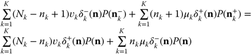
where  ,
,  and
and ![]() are the probability distributions of the corresponding states
are the probability distributions of the corresponding states ![]() , and
, and ![]() , respectively.
, respectively.

Figure 6.3 State transition diagram of the EnMLM.
Assume now the existence of LB between adjacent states. Equations (6.23) and (6.24) are the detailed LB equations which hold (for ![]() and
and ![]() ) because the Markov chain of the EnMLM is reversible:
) because the Markov chain of the EnMLM is reversible:
Based on the LB assumption, the probability distribution ![]() has the following PFS [3]:
has the following PFS [3]:

where ![]() is the offered traffic‐load per idle source of service‐class
is the offered traffic‐load per idle source of service‐class ![]() ,
, ![]() is the normalization constant given by
is the normalization constant given by  , and
, and ![]() .
.
If we denote by ![]() the occupied link bandwidth (
the occupied link bandwidth (![]() ) then the link occupancy distribution,
) then the link occupancy distribution, ![]() , is defined as:
, is defined as:

where ![]() is the set of states whereby exactly
is the set of states whereby exactly ![]() b.u. are occupied by all in‐service calls, i.e.,
b.u. are occupied by all in‐service calls, i.e., ![]() .
.
The unnormalized values of ![]() can be recursively determined by [ 3]:
can be recursively determined by [ 3]:

Note that if ![]() for
for ![]() , and the total offered traffic‐load remains constant, then we have the Kaufman–Roberts recursion (1.39) of the EMLM.
, and the total offered traffic‐load remains constant, then we have the Kaufman–Roberts recursion (1.39) of the EMLM.
Summing both sides of (6.28) over ![]() we have:
we have:

The LHS of (6.29) is written as ![]() . Since
. Since  and based on (1.47), we may write the LHS of ( 6.29) as follows [ 3]:

The term ![]() is written as
is written as ![]() , while the term
, while the term ![]() is written as
is written as ![]() , where
, where ![]() is the mean number of service‐class
is the mean number of service‐class ![]() calls in state
calls in state ![]() . Then, (6.30) (i.e., the LHS of ( 6.29)) can be written as:
. Then, (6.30) (i.e., the LHS of ( 6.29)) can be written as:

The RHS of ( 6.29) is written as:

By equating (6.31) and (6.32) (because of ( 6.29)), we have:
Multiplying both sides of (6.33) by ![]() and summing over
and summing over ![]() we have:
we have:

The value of ![]() in (6.34) is not known. To determine it, we use a lemma proposed in [ 3]. According to the lemma, two stochastic systems are equivalent and result in the same CBP if they have: (a) the same traffic description parameters
in (6.34) is not known. To determine it, we use a lemma proposed in [ 3]. According to the lemma, two stochastic systems are equivalent and result in the same CBP if they have: (a) the same traffic description parameters ![]() where
where ![]() , and (b) exactly the same set of states.
, and (b) exactly the same set of states.
The purpose is therefore to find a new stochastic system in which we can determine the value ![]() . The bandwidth requirements of calls of all service‐classes and the capacity
. The bandwidth requirements of calls of all service‐classes and the capacity ![]() in the new stochastic system are chosen according to the following two criteria:
in the new stochastic system are chosen according to the following two criteria:
(i) conditions (a) and (b) are valid, and (ii) each state has a unique occupancy j.
Now, state j is reached only via the previous state ![]() . Thus,
. Thus, ![]() .
.
Based on the above, ( 6.34) can be written as ( 6.27).
Q.E.D.
6.2.2.2 TC Probabilities, CBP, Utilization, and Mean Number of In‐service Calls
The following performance measures can be determined based on ( 6.27):
- The TC probabilities of service‐class
 , via:
(6.35)where
, via:
(6.35)where
 is the normalization constant.
 - The CBP (or CC probabilities) of service‐class
 , via (6.35) but for a system with
  traffic sources.
 - The link utilization,
 , via:
(6.36)
, via:
(6.36)
- The average number of service‐class
 calls in the system,
  , via:
(6.37)where
, via:
(6.37)where
 is the average number of service‐class
  calls given that the system state is
  , and is given by:
(6.38)where
, and is given by:
(6.38)where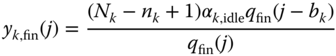
 , while
  for
for  and
and  .
.
The determination of ![]() via ( 6.27), and consequently of all performance measures, requires the value of
via ( 6.27), and consequently of all performance measures, requires the value of ![]() , which is unknown. In [ 3], there exists a method for the determination of
, which is unknown. In [ 3], there exists a method for the determination of ![]() in each state
in each state ![]() via an equivalent stochastic system, with the same traffic parameters and the same set of states as already described for the proof of ( 6.27). This method results in the accurate calculation of
via an equivalent stochastic system, with the same traffic parameters and the same set of states as already described for the proof of ( 6.27). This method results in the accurate calculation of ![]() . However, the state space determination of the equivalent system is complex, especially for large capacity systems that serve many service‐classes.
. However, the state space determination of the equivalent system is complex, especially for large capacity systems that serve many service‐classes.
6.2.2.3 An Approximate Algorithm for the Determination of 
Contrary to ( 6.27), which provides the exact values of the various performance measures, at the cost of state space enumeration and processing, the algorithm presented herein provides approximate values but is much simpler and easy to implement, therefore it is adopted in the forthcoming finite multirate loss models presented in this chapter and the following chapters.
The algorithm comprises the following steps [4]:

6.3 The Engset Multirate Loss Model under the BR Policy
6.3.1 The Service System
We consider again the system of the EnMLM and apply the BR policy (EnMLM/BR): A new service‐class k call is accepted in the link if, after its acceptance, the occupied link bandwidth ![]() , where
, where ![]() refers to the BR parameter used to benefit calls of all other service‐classes apart from k (see also the EMLM/BR in Section 1.3.1).
refers to the BR parameter used to benefit calls of all other service‐classes apart from k (see also the EMLM/BR in Section 1.3.1).
In terms of the system state‐space ![]() , the CAC is expressed as follows. A new call of service‐class k is accepted in the system if the system is in state
, the CAC is expressed as follows. A new call of service‐class k is accepted in the system if the system is in state ![]() upon a new call arrival, where
upon a new call arrival, where ![]() . Hence, the TC probabilities of service‐class k are determined by the state space
. Hence, the TC probabilities of service‐class k are determined by the state space ![]() (see ( 6.21)).
(see ( 6.21)).
As far as the CC probabilities, ![]() , are concerned, they can be determined by ( 6.21) as well but for a system with
, are concerned, they can be determined by ( 6.21) as well but for a system with ![]() traffic sources.
traffic sources.
6.3.2 The Analytical Model
6.3.2.1 Link Occupancy Distribution
In the EnMLM/BR, the unnormalized values of ![]() can be calculated in an approximate way according to the Roberts method (see Section 1.3.2.2). Based on this method, we can either find an equivalent stochastic system (which requires enumeration and processing of the state space) [5] or apply an algorithm similar to that presented in Section 6.2.2.3 [6]. Due to its simplicity, we adopt the algorithm of [ 6], which is described by the following steps:
can be calculated in an approximate way according to the Roberts method (see Section 1.3.2.2). Based on this method, we can either find an equivalent stochastic system (which requires enumeration and processing of the state space) [5] or apply an algorithm similar to that presented in Section 6.2.2.3 [6]. Due to its simplicity, we adopt the algorithm of [ 6], which is described by the following steps:

6.3.2.2 TC Probabilities, CBP, Utilization, and Mean Number of In‐service Calls
The following performance measures can be determined based on (6.41):
- The TC probabilities of service‐class
 , via:
(6.42)where
, via:
(6.42)where
 is the normalization constant.
 - The CBP (or CC probabilities) of service‐class
 , via (6.42) but for a system with
  traffic sources.
 - The link utilization, U, via (6.36).
- The average number of service‐class k calls in the system,
 , via (6.37), while:
(6.43)
, via (6.37), while:
(6.43)
6.4 The Engset Multirate Loss Model under the TH Policy
6.4.1 The Service System
We consider the multiservice system of the EnMLM under the TH policy (![]() ). The call admission is exactly the same as that of the EMLM/TH (see Section 1.4.1).
). The call admission is exactly the same as that of the EMLM/TH (see Section 1.4.1).
6.4.2 The Analytical Model
6.4.2.1 Steady State Probabilities
Since the TH policy is a coordinate convex policy the steady state probabilities in the EnMLM/TH have a PFS whose form is exactly the same as that of the EnMLM (the only change is in the definition of ![]() ):
):

where ![]() is the offered traffic‐load per idle source of service‐class
is the offered traffic‐load per idle source of service‐class ![]() ,
, ![]() is the normalization constant given by
is the normalization constant given by  , and
, and ![]() .
.
Equation (6.44) satisfies the GB equation of (6.22) and the LB equations of ( 6.23) and ( 6.24), while the state transition diagram of the EnMLM/TH is the same as in Figure 6.3.
In order to determine the TC probabilities of service‐class k, ![]() , we denote by
, we denote by ![]() the admissible state space of service‐class k:
the admissible state space of service‐class k: ![]() , where
, where ![]() and
and ![]() . A new service‐class k call is accepted in the system if, at the time point of its arrival, the system is in a state
. A new service‐class k call is accepted in the system if, at the time point of its arrival, the system is in a state ![]() . Hence, the TC probabilities of service‐class k are determined by the state space
. Hence, the TC probabilities of service‐class k are determined by the state space ![]() and according to ( 6.21).
and according to ( 6.21).
Following the analysis of the EnMLM for the determination of ![]() and the analysis of the EMLM/TH it can be proved that the values of
and the analysis of the EMLM/TH it can be proved that the values of ![]() are given by [7]:
are given by [7]:

where ![]() is the probability that x b.u. are occupied, while the number of service‐class k calls is
is the probability that x b.u. are occupied, while the number of service‐class k calls is ![]() or:
or:
Equation (6.45) requires knowledge of ![]() . The latter takes positive values when
. The latter takes positive values when ![]() . Thus, we consider a subsystem of capacity
. Thus, we consider a subsystem of capacity ![]() that accommodates all service‐classes but service‐class k. For this subsystem, we define
that accommodates all service‐classes but service‐class k. For this subsystem, we define ![]() , which is analogous to
, which is analogous to ![]() of ( 6.45):
of ( 6.45):

We can now compute ![]() when
when ![]() , as follows:
, as follows:

In (6.48), the term  is expected, since for states
 ![]() , the number of in‐service calls of service‐class k is always
, the number of in‐service calls of service‐class k is always ![]() .
.
If ![]() for
for ![]() and the total offered traffic‐load remains constant, then ( 6.45), (6.47), and ( 6.48) become (1.73), (1.78), and (1.79), respectively, of the EMLM/TH.
and the total offered traffic‐load remains constant, then ( 6.45), (6.47), and ( 6.48) become (1.73), (1.78), and (1.79), respectively, of the EMLM/TH.
Equations ( 6.45) and ( 6.47) require an equivalent stochastic system in order for the various performance measures to be determined, given that the values of ![]() are unknown. An alternative procedure is an algorithm similar to that presented in Section 6.2.2.3 [ 7]:
are unknown. An alternative procedure is an algorithm similar to that presented in Section 6.2.2.3 [ 7]:

6.4.2.2 CBP, Utilization and Mean Number of In‐service Calls
The following performance measures can be determined based on (6.49):
- The TC probabilities of service‐class
 , via:
(6.52)where
, via:
(6.52)where
 is the normalization constant.
 - The CBP (or CC probabilities) of service‐class
 , via (6.52) but for a system with
  traffic sources.
 - The link utilization, U, via ( 6.36).
- The average number of service‐class k calls in the system,
 , via ( 6.37) where
  are given by:
(6.53)
are given by:
(6.53)
6.5 Applications
In order to remember a typical application example of a simple Engset system, it is worth mentioning that Example 6.2 could correspond to an office (in a company) accommodating four clerks with a telephone set dedicated to each clerk, while the four telephone sets equally share two telephone lines.
A recent application of the EnMLM has been proposed in [8] for the calculation of TC and CC probabilities in the X2 link of LTE networks. The main components of an LTE network are the evolved packet core (EPC) and the evolved terrestrial radio access network (E‐UTRAN). The EPC is responsible for the management of the core network components and the communication with the external network. The E‐UTRAN provides air interface, via evolved NodeBs (eNBs), to user equipment (UE) and acts as an intermediate node handling the radio communication between the UE and the EPC. Each eNB covers a specific cell and exchanges traffic with the core network through the S1 interface. An active UE is quite likely to cross the boundary of the source cell, causing a handover. A handover is the process of a seamless transition of the UE's radio link from the source eNB to one of its neighbors. During this transition, the direct logical interface (link) between two neighboring eNBs – the X2 link – is used for the user data arriving to the source eNB via the S1 link to be transferred to the target eNB (Figure 6.12).

Figure 6.12 The S1 interface and the X2 interface between source and target eNBs.
The determination of congestion probabilities in the X2 link can be based on the following multirate teletraffic loss model. Consider the X2 link of fixed capacity ![]() that accommodates
that accommodates ![]() different service‐classes. Calls of service class
different service‐classes. Calls of service class ![]() require
require ![]() channels and come from a finite source population
channels and come from a finite source population ![]() , while the mean arrival rate of service‐class
, while the mean arrival rate of service‐class ![]() idle sources is
idle sources is ![]() , where
, where ![]() is the number of in‐service calls and
is the number of in‐service calls and ![]() is the arrival rate per idle source. To determine the offered traffic‐load in the X2 link, the fluid mobility model of [9] is adopted in which traffic flow is considered as the flow of a fluid. Such a model can be used to model the behavior of macroscopic movement (i.e., the movement of an individual UE is considered of little significance) [10]. This fluid mobility model formulates the amount of traffic flowing out of a circular region of a source cell to be proportional to the population density within that region, the average velocity, and the length of the region boundary. More precisely, assuming a population density1 of
is the arrival rate per idle source. To determine the offered traffic‐load in the X2 link, the fluid mobility model of [9] is adopted in which traffic flow is considered as the flow of a fluid. Such a model can be used to model the behavior of macroscopic movement (i.e., the movement of an individual UE is considered of little significance) [10]. This fluid mobility model formulates the amount of traffic flowing out of a circular region of a source cell to be proportional to the population density within that region, the average velocity, and the length of the region boundary. More precisely, assuming a population density1 of ![]() for a circular source cell of radius
for a circular source cell of radius ![]() and that the UEs are always active, then the total offered traffic load of service‐class
and that the UEs are always active, then the total offered traffic load of service‐class ![]() is
is ![]() , where
, where ![]() is the average velocity of service‐class
is the average velocity of service‐class ![]() UEs and
UEs and ![]() is the interruption time (in the order of 50 ms) of the radio link between the source eNB and the UE. Then, the offered traffic‐load per idle source of service‐class
is the interruption time (in the order of 50 ms) of the radio link between the source eNB and the UE. Then, the offered traffic‐load per idle source of service‐class ![]() is given by
is given by ![]() (in erl). Now, the determination of CC and TC probabilities of service‐class
(in erl). Now, the determination of CC and TC probabilities of service‐class ![]() in the X2 link can be based on the EnMLM [ 8].
in the X2 link can be based on the EnMLM [ 8].
Another interesting application of the EnMLM on smart grid is proposed in [11]. The authors of [ 11] propose four power demand control scenarios that correspond to different approaches on the control of power customers' power demands. All scenarios assume that in each residence a specific number of appliances is installed, with diverse power requirements, different operational times, and different power requests arrival rates. Of course, a finite number of appliances in the whole residential area is considered. This consideration is expressed by a quasi‐random process for the procedure of arrivals of power requests, which is more realistic compared to the Poisson process (infinite number of power‐request sources). A short description of the four scenarios is as follows:
- (i) The default scenario defines the upper bound of the total power consumption, since it does not consider any scheduling mechanism.
- (ii) The compressed demand scenario takes into account the ability of some appliances to compress their power demands and at the same time expand their operational times.
- (iii) In the delay request scenario, power requests are delayed in buffers for a specific time period, when the total power consumption exceeds a predefined threshold.
- (iv) In the postponement request scenario, a similar threshold is used where power requests are postponed not for a specific time period, but until the total power consumption drops below a second threshold.
6.6 Further Reading
Regarding an in‐depth theoretical analysis of the Engset loss model, the interested reader may refer to [12,13]. In [ 12], recursive formulas for the determination of CC and TC probabilities are proposed which resemble the recurrent form of the Erlang‐B formula. In [ 13], the Engset loss model is extended to include a fractional number of sources and servers.
A quite interesting work whose springboard is the Engset loss model is [14], which is known in the literature as the generalized Engset model. In [ 14], two generalizations are considered: (i) the distributions of the service (holding) time and interarrival time may differ from source to source and (ii) the idle time distribution may depend on whether or not the previous call was accepted in the system. For applications of the generalized Engset model or extensions of [ 14], the interested reader may refer to [15–20].
Regarding the EnMLM, several extensions appear in the literature covering wired [21–24], wireless [25–31], and optical [32,33] networks. In [ 21], an analytical method is proposed for the CBP calculation in switching networks accommodating multirate random and quasi‐random traffic. In [22], an analytical model is proposed for the determination of TC and CC probabilities in a single link accommodating multirate quasi‐random traffic under a reservation policy in which the reserved b.u. can have a real (not integer) value. In [23], an analytical model is proposed for the point‐to‐point blocking probability calculation in switching networks with multicast connections. In [ 24], an analytical model is proposed for the determination of blocking probabilities in a switching network carrying Erlang, Engset, and Pascal multirate traffic under different resource allocation control mechanisms. In [ 25–27], the EnMLM is extended to become suitable for the analysis of WCDMA networks. In [ 25], the authors incorporate in the model the notion of intra‐ and inter‐cell interference as well as the noise rise and user's activity. A generalization of [ 25] appears in [26] where handover traffic is explicitly distinguished from new traffic. In [ 27], a different model is proposed that takes into account not only the uplink (as in [ 25, 26]) but also the downlink direction. In [28], a time division multiple access/frequency division duplexing (TDMA/FDD) based medium access control (MAC) protocol is proposed for broadband wireless networks that accommodate real‐time multimedia applications. The CAC in the proposed MAC is based on the CS policy while the CBP determination is achieved via the EnMLM. In [29], the benefits of software‐defined networking (SDN) on the radio resource management (RRM) of future‐generation cellular networks are studied. The aim of the proposed RRM scheme is to enable the macro BS to efficiently allocate radio resources for small cell BSs in order to assure QoS of moving users/vehicles during handoffs. To this end, an approximate, but very time‐ and space‐efficient, algorithm for radio resource allocation within a heterogeneous network is proposed based on the EnMLM. In [30], a teletraffic model is proposed for the call‐level analysis of priority‐based cellular CDMA networks that accommodate multiple service‐classes with finite source population. In [ 31], various state‐dependent bandwidth sharing policies are presented and efficient formulas for the CBP determination are proposed for wireless multirate loss networks. In [ 32], teletraffic loss models are proposed for the calculation of connection failure probabilities (due to unavailability of a wavelength) and CBP (due to the restricted bandwidth capacity of a wavelength) in hybrid TDM‐WDM PONs with dynamic wavelength allocation. EMLM and the EnMLM form the springboard of the analysis. Finally, in [ 33], the EnMLM is used for the determination of blocking probabilities in WDM dynamic networks operating with alternate routing.
References
- 1 H. Akimaru and K. Kawashima, Teletraffic – Theory and Applications, 2nd edn, Springer, Berlin, 1999.
- 2 E. Pinsky, A. Conway and W. Liu, Blocking formulae for the Engset model. IEEE Transactions on Communications, 42(6):2213–2214, June 1994.
- 3 G. Stamatelos and J. Hayes, Admission control techniques with application to broadband networks. Computer Communications, 17(9):663–673, September 1994.
- 4 M. Glabowski and M. Stasiak, An approximate model of the full‐availability group with multi‐rate traffic and a finite source population. Proceedings of the 12th MMB&PGTS, Dresden, Germany, September 2004.
- 5 I. Moscholios and M. Logothetis, Engset multirate state‐dependent loss models with QoS guarantee. International Journal of Communications Systems, 19(1):67–93, February 2006.
- 6 M. Glabowski, Modelling of state‐dependent multirate systems carrying BPP traffic. Annals of Telecommunications, 63(7–8):393–407, August 2008.
- 7 I. Moscholios, M. Logothetis, J. Vardakas and A. Boucouvalas, Performance metrics of a multirate resource sharing teletraffic model with finite sources under both the threshold and bandwidth reservation policies. IET Networks, 4(3):195–208, May 2015.
- 8 P. Panagoulias, I. Moscholios, M. Koukias and M. Logothetis, A multirate loss model of quasi‐random input for the X2 link of LTE networks. Proceedings of the 17th International Conference on Networks (ICN), Athens, Greece, April 2018.
- 9 I. Widjaja and H. La Roche, Sizing X2 bandwidth for inter‐connected eNBs. Proceedings of the IEEE VTC Fall, Anchorage, Alaska, USA, pp. 1–5, September 2009.
- 10 D. Lam, D. Cox and J. Widom, Teletraffic modeling for personal communications services. IEEE Communications Magazine, 35(2):79–87, February 1997.
- 11 J. Vardakas, N. Zorba and C. Verikoukis, Power demand control scenarios for smart grid applications with finite number of appliances. Applied Energy, 162, 83–98, January 2016.
- 12 E. Pinsky, A. Conway and W. Liu, Blocking formulae for the Engset model. IEEE Transactions on Communications, 42(6): 2213–2214, June 1994.
- 13 V. Iversen and B. Sanders, Engset formulae with continuous parameters: theory and applications. International Journal of Electronics and Communications, 55(1): 3–9, 2001.
- 14 J.W. Cohen, The generalized Engset formulae. Philips Telecommunication Review, 18(4): 158–170, 1957.
- 15 J. Karvo, O. Martikainen, J. Virtamo and S. Aalto, Blocking of dynamic multicast connections. Telecommunication Systems, 16(3–4):467–481, March 2001.
- 16 H. Kobayashi and B. Mark, Generalized loss models and queueing loss networks. International Transactions in Operational Research, 9(1):97–112, January 2002.
- 17 E. Wong, A. Zalesky and M. Zukerman, A state‐dependent approximation for the generalized Engset model. IEEE Communications Letters, 13(2):962–964, December 2009.
- 18 Y. Deng and P. Prucnal, Performance analysis of heterogeneous optical CDMA networks with bursty traffic and variable power control. IEEE/OSA Journal of Optical Communications and Networking, 3(6):487–492, June 2011.
- 19 J. Zhang, Y. Peng, E. Wong and M. Zukerman, Sensitivity of blocking probability in the generalized Engset model for OBS. IEEE Communications Letters, 15(11):1243–1245, November 2011.
- 20 J. Zhang and L. Andrew, Efficient generalized Engset blocking calculation. IEEE Communications Letters, 18(9):1535–1538, September 2014.
- 21 M. Glabowski and M. Stasiak, Internal blocking probability calculation in switching networks with additional inter‐stage links and mixture of Erlang and Engset traffic. Image Processing & Communications, 17(1–2):67–80, June 2012.
- 22 I. Moscholios, Congestion probabilities in Erlang–Engset multirate loss models under the multiple fractional channel reservation policy. Image Processing & Communications, 21(1):35–46, 2016.
- 23 M. Sobieraj and P. Zwierzykowski, Blocking probability in switching networks with multi‐service sources and multicast traffic. Proceedings of the IEEE CSNDSP, Prague, Czech Republic, July 2016.
- 24 M. Glabowski and M. Sobieraj, Analytical modelling of multiservice switching networks with multiservice sources and resource management mechanisms. Telecommunication Systems, 66(3):559–578, November 2017.
- 25 V. Vassilakis, G. Kallos, I. Moscholios and M. Logothetis, The wireless Engset multi‐rate loss model for the call‐level analysis of W‐CDMA networks. Proceedings of the 18th Annual IEEE International Symposium on Personal, Indoor and Mobile Radio Communications, PIMRC 07, Athens, Greece, September 2007.
- 26 V. Vassilakis, G. Kallos, I. Moscholios and M. Logothetis, On call admission control in W‐CDMA networks supporting handoff traffic. Ubiquitous Computing and Communication Journal, Special Issue on IEEE CSNDSP 2008, September 2009.
- 27 M. Glabowski, M. Stasiak, A. Wisniewski and P. Zwierzykowski, Blocking probability calculation for cellular systems with WCDMA radio interface servicing PCT1 and PCT2 multirate traffic. IEICE Transactions on Communications, E92‐B(4):1156–1165, April 2009.
- 28 S. Atmaca, A. Karahan, C. Ceken and I. Erturk, A new MAC protocol for broadband wireless communications and its performance evaluation. Telecommunication Systems, 57(1):13–23, September 2014.
- 29 V. Vassilakis, I. Moscholios, A. Bontozoglou and M. Logothetis, Mobility‐aware QoS assurance in software‐defined radio access networks: An analytical study. Proceedings of the IEEE International Workshop on Software Defined 5G Networks, London, UK, April 2015.
- 30 V. Vassilakis, I. Moscholios and M. Logothetis, Uplink blocking probabilities in priority‐based cellular CDMA networks with finite source population. IEICE Transactions on Communications, E99‐B(6):1302–1309, June 2016.
- 31 I. Moscholios, V. Vassilakis, M. Logothetis and A. Boucouvalas, State‐dependent bandwidth sharing policies for wireless multirate loss networks. IEEE Transactions on Wireless Communications, 16(8):5481–5497, August 2017.
- 32 J. Vardakas, V. Vassilakis and M. Logothetis, Blocking analysis in hybrid TDM‐WDM passive optical networks, in Performance Modelling and Analysis of Heterogeneous Networks, D. Kouvatsos (ed.), River Publishers, pp. 441–465, 2009.
- 33 N. Jara and A. Beghelli, Blocking probability evaluation of end‐to‐end dynamic WDM networks. Photonic Network Communications, 24(1):29–38, August 2012.