2
Multirate Retry Threshold Loss Models
We consider multirate loss models of random arriving calls with elastic bandwidth requirements and fixed bandwidth allocation during service. Calls may retry several times upon arrival (requiring less bandwidth each time) in order to be accepted for service. Alternatively, calls may request less bandwidth upon arrival, according to the occupied link bandwidth indicated by threshold(s).
2.1 The Single‐Retry Model
2.1.1 The Service System
In the single‐retry model (SRM), a link of capacity ![]() b.u. accommodates Poisson arriving calls of
b.u. accommodates Poisson arriving calls of ![]() service‐classes, under the CS policy. A new call of service‐class
service‐classes, under the CS policy. A new call of service‐class ![]() has a peak‐bandwidth requirement of
has a peak‐bandwidth requirement of ![]() b.u. and an exponentially distributed service time with mean
b.u. and an exponentially distributed service time with mean ![]() . If the initially required b.u. are not available in the link, the call is blocked, but immediately retries to be connected with bandwidth requirement
. If the initially required b.u. are not available in the link, the call is blocked, but immediately retries to be connected with bandwidth requirement ![]() b.u., while the mean of the new (exponentially distributed) service time increases to
b.u., while the mean of the new (exponentially distributed) service time increases to ![]() , so that the product bandwidth requirement by service time
, so that the product bandwidth requirement by service time ![]() remains constant [1,2]. If the
remains constant [1,2]. If the ![]() b.u. are not available, the call is blocked and lost (Figure 2.1). The CAC mechanism of a call of service‐class
b.u. are not available, the call is blocked and lost (Figure 2.1). The CAC mechanism of a call of service‐class ![]() is depicted in Figure 2.2. A new call of service‐class
is depicted in Figure 2.2. A new call of service‐class ![]() is blocked with
is blocked with ![]() b.u. if
b.u. if ![]() and is accepted with
and is accepted with ![]() b.u., if
b.u., if ![]() , where
, where ![]() and
and ![]() are the in‐service calls of service‐class
are the in‐service calls of service‐class ![]() (in the steady state of the system) accepted with
(in the steady state of the system) accepted with ![]() b.u., respectively. The comparison of the SRM with the EMLM reveals the following basic differences:
b.u., respectively. The comparison of the SRM with the EMLM reveals the following basic differences:
- (i) The steady state probabilities in the SRM do not have a PFS, since the notion of LB between adjacent states does not hold (see Example 2.1). Because of this, the unnormalized values of
 are determined via an approximate, but recursive, formula, as Section 2.1.2 shows.
 - (ii) In the EMLM, the steady state vector of all in‐service calls of all service‐classes is
 , while in the SRM the corresponding vector becomes
  . This dimensionality increase means that only quite small problems can be solved exactly (see Example 2.1).
 - (iii) In the EMLM, the calculation of
 via the Kaufman–Roberts recursion (1.39) is insensitive to the service time distribution [3]. In the SRM, this insensitivity property does not hold. However, numerical examples in [ 2] show that the CBP obtained for various service time distributions are quite close.

Figure 2.1 Service system of the SRM.

Figure 2.2 The CAC mechanism for a new call in the SRM.

Figure 2.3 The state space  (CS policy) and the state transition diagram (Example 2.1).
2.1.2 The Analytical Model
2.1.2.1 Steady State Probabilities
To describe the analytical model in the steady state, let us concentrate on a single link of capacity ![]() b.u. that accommodates two service‐classes with the following traffic characteristics:
b.u. that accommodates two service‐classes with the following traffic characteristics: ![]() . Blocked calls of service‐class 2 can retry with parameters
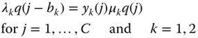
. Blocked calls of service‐class 2 can retry with parameters ![]() , while blocked calls of service‐class 1 are not allowed to retry. Although the SRM does not have a PFS, we assume that the LB equation (1.51) proposed in the EMLM does hold, that is:
, while blocked calls of service‐class 1 are not allowed to retry. Although the SRM does not have a PFS, we assume that the LB equation (1.51) proposed in the EMLM does hold, that is:
This assumption (approximation) is important for the derivation of an approximate but recursive formula for the calculation of ![]() . The aforementioned equation expresses the fact that no call blocking occurs in state
. The aforementioned equation expresses the fact that no call blocking occurs in state ![]() , if there are available
, if there are available ![]() b.u.
b.u. ![]() . If
. If ![]() , when a new call of service‐class 2 arrives in the system, then this call is blocked and retries to be connected with
, when a new call of service‐class 2 arrives in the system, then this call is blocked and retries to be connected with ![]() b.u. If
b.u. If ![]() , then, the retry call will be accepted in the system. To describe the latter case, we need an additional LB equation [ 2]:
, then, the retry call will be accepted in the system. To describe the latter case, we need an additional LB equation [ 2]:

where ![]() is the mean number of service‐class
is the mean number of service‐class ![]() calls accepted in the system with
calls accepted in the system with ![]() in state
in state ![]() .
.
Dividing (2.2) by ![]() and multiplying by
and multiplying by ![]() , we obtain [ 2]:
, we obtain [ 2]:

where ![]() is the offered traffic‐load of service‐class 2 calls with
is the offered traffic‐load of service‐class 2 calls with ![]() .
.
Equation (2.1) can be written as ![]() . Then, by multiplying both sides with
. Then, by multiplying both sides with ![]() and summing up for
and summing up for ![]() , we have:
, we have:

Adding (2.3) to (2.4), and since ![]() , we have:
, we have:

Apart from the assumption of the LB equation ( 2.1), another approximation is necessary for the recursive calculation of ![]() [ 2]:
[ 2]:

Equation (2.6) expresses the so‐called migration approximation [ 1, 2,4], according to which the number of calls accepted in the system with other than the maximum bandwidth requirement is negligible within a state space, called the migration space. In this space, the value of ![]() is negligible compared to
is negligible compared to ![]() when
when ![]() . For service‐class
. For service‐class ![]() (with
(with ![]() ):
):

Equation ( 2.4) due to ( 2.6) is written as:

The combination of (2.5) and (2.8) is achieved through the use of a binary parameter (![]() ), and gives an approximate but recursive formula for the determination of
), and gives an approximate but recursive formula for the determination of ![]() in the SRM, considering two service‐classes where only calls of service‐class 2 can retry [ 1, 2]:
in the SRM, considering two service‐classes where only calls of service‐class 2 can retry [ 1, 2]:
where ![]() , and
, and ![]() when
when ![]() (otherwise
(otherwise ![]() ).
).
The symbol ![]() is used to distinguish retry models, where only the migration approximation exists, from other models (e.g., thresholds models presented in Section 2.5) where the symbol
is used to distinguish retry models, where only the migration approximation exists, from other models (e.g., thresholds models presented in Section 2.5) where the symbol ![]() is used and additional approximations are considered.
is used and additional approximations are considered.
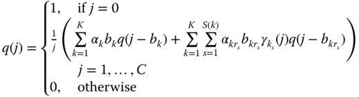
The generalization of (2.9) for ![]() service‐classes, where all service‐classes may retry, is as follows [ 2]:
service‐classes, where all service‐classes may retry, is as follows [ 2]:

where ![]() and
and ![]() when
when ![]() (otherwise
(otherwise ![]() ).
).
Note that the variable ![]() in (2.10) expresses the migration approximation, i.e., (2.7).
in (2.10) expresses the migration approximation, i.e., (2.7).
2.1.2.2 CBP, Utilization, and Mean Number of In‐service Calls
Having determined the unnormalized values of ![]() , we can calculate the following performance measures:
, we can calculate the following performance measures:
- The CBP of service‐class
 calls with
  b.u. (i.e., the actual CBP of service‐class
  with retrial),
  , via the following formula [ 2]:
(2.11)where
, via the following formula [ 2]:
(2.11)where
 is the normalization constant.
 - The CBP of service‐class
 calls with
  b.u. (i.e., the actual CBP of service‐class
  without retrial, or the retry probability in case of service‐class
  with retrial),
  , via:
(2.12)
, via:
(2.12)
- The conditional CBP of service‐class
 retry calls given that they have been blocked with their initial bandwidth requirement
  , via:
(2.13)
, via:
(2.13)
- The link utilization,
 , via (1.54).
 - The mean number of service‐class k calls with
 b.u. in state
  , via:
(2.14)
, via:
(2.14)
- The mean number of service‐class
 calls with
  b.u. in state
  , via:
(2.15)where
, via:
(2.15)where
 when
when  (otherwise
  ).
). - The mean number of in‐service calls of service‐class k accepted in the system with
 , via:
(2.16)
, via:
(2.16)
- The mean number of in‐service calls of service‐class k accepted in the system with
 , via:
(2.17)
, via:
(2.17)
2.2 The Single‐Retry Model under the BR Policy
2.2.1 The Service System
In the SRM under the BR policy (SRM/BR), ![]() b.u. are reserved to benefit calls of all other service‐classes apart from service‐class
b.u. are reserved to benefit calls of all other service‐classes apart from service‐class ![]() . The application of the BR policy in the SRM is similar to that of the EMLM/BR, as the following example shows.
. The application of the BR policy in the SRM is similar to that of the EMLM/BR, as the following example shows.
2.2.2 The Analytical Model
2.2.2.1 Steady State Probabilities
To calculate the link occupancy distribution in the steady state of the SRM/BR, we prefer the Roberts method to the Stasiak–Glabowski method. The latter is more complex compared to the Roberts method and does not provide more accurate results (compared to simulation) in retry loss models and threshold loss models (see Section 2.6, below) [5].
Based on the Roberts method, ( 2.10) takes the form [ 4]:

where ![]() ,
, ![]() , when
, when ![]() (otherwise
(otherwise ![]() ),
), ![]() is given by (1.65) and, similarly,
is given by (1.65) and, similarly, ![]() by:
by:

2.2.2.2 CBP, Utilization, and Mean Number of In‐service Calls
Based on (2.18) and (2.19), we can calculate the following performance measures:
- The CBP of service‐class
 calls with
  b.u.,
b.u.,  , via the following formula [ 4]:
(2.20)where
, via the following formula [ 4]:
(2.20)where
 is the normalization constant.
 - The CBP of service‐class
 calls with
  b.u.,
b.u.,  (i.e., the actual CBP of service‐class
  without retrials, or retry probability in case of service‐class
  with retrials), can be determined via (1.66), while the conditional CBP of service‐class
  retry calls given that they have been blocked with their initial bandwidth requirement
  , via (2.13), while subtracting
  from
from  and from
  .
. - The link utilization,
 , is given by (1.54).
 - The mean number of service‐class
 calls with
  b.u. in state
  ,
,  , is given by (1.67), while the mean number of service‐class
  calls with
  b.u. in state
  ,
,  , is given by:
(2.21)where
, is given by:
(2.21)where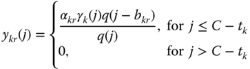
 when
when  (otherwise
  ).
). - The mean number of in‐service calls of service‐class
 accepted in the system with
  , is calculated by (2.16), while the mean number of in‐service calls of service‐class
  accepted in the system with
  , by (2.17).
Table 2.1 CBP of Example 2.5 (SRM, ![]() b.u. and
b.u. and ![]() b.u.).
b.u.).
| CBP | Analytical results | Simulation results | Analytical results | Simulation results |
| 0.0479 | 0.0493 |
0.0004 | 0.0004 |
|
| 0.2997 | 0.2986 |
0.0031 | 0.0029 |
|
| 0.5089 | 0.5077 |
0.0063 | 0.0060 |
|
| 0.7360 | 0.7430 |
0.0128 | 0.0125 |
|
| 0.5089 | 0.5081 |
0.0063 | 0.0060 |
|
| 0.6914 | 0.6844 |
0.4955 | 0.4871 |
|
Table 2.2 CBP of Example 2.5 (SRM/BR, ![]() b.u. and
b.u. and ![]() b.u.).
b.u.).
| CBP | Analytical results | Simulation results | Analytical results | Simulation results |
| 0.3804 | 0.3825 |
0.00485 | 0.00485 |
|
| 0.3804 | 0.3826 |
0.00485 | 0.00486 |
|
| 0.3804 | 0.3824 |
0.00485 | 0.00485 |
|
| 0.3804 | 0.3825 |
0.00485 | 0.00487 |
|

Figure 2.5 CBP in the SRM and EMLM, for various values of  (Example 2.5).

Figure 2.6 Link utilization in the SRM and EMLM (Example 2.5).

Figure 2.7 CBP in the SRM/BR and the EMLM/BR for various values of  (Example 2.5).
2.3 The Multi‐Retry Model
2.3.1 The Service System
In the multi‐retry model (MRM), calls of service‐class ![]() can retry not only once, but several times, in order to be accepted in the system [ 1, 2]. Let
can retry not only once, but several times, in order to be accepted in the system [ 1, 2]. Let ![]() be the number of retrials for calls of service‐class
be the number of retrials for calls of service‐class ![]() , and assume that
, and assume that ![]() , where
, where ![]() is the required bandwidth of a service‐class
is the required bandwidth of a service‐class ![]() call in the
call in the ![]() retry,
retry, ![]() . Then a service‐class
. Then a service‐class ![]() call is accepted in the system with
call is accepted in the system with ![]() b.u. if
b.u. if ![]() . By definition,
. By definition, ![]() and
and ![]() .
.
2.3.2 The Analytical Model
2.3.2.1 Steady State Probabilities
Following the analysis of Section 2.1.2.1, we have to assume in the MRM the existence of both LB and the migration approximation. According to the migration approximation, the mean number of service‐class k calls in state ![]() ,
, ![]() , accepted with
, accepted with ![]() b.u., is negligible when
b.u., is negligible when ![]() , where
, where ![]() . This means that service‐class k calls with
. This means that service‐class k calls with ![]() are limited in the area
are limited in the area ![]() . Based on [1, 2], the unnormalized values of
. Based on [1, 2], the unnormalized values of ![]() can be determined by the following recursive formula:
can be determined by the following recursive formula:
where ![]() when
when ![]() (otherwise
(otherwise ![]() ).
).
2.3.2.2 CBP, Utilization, and Mean Number of In‐service Calls
Having determined the unnormalized values of ![]() , we can determine the following performance measures:
, we can determine the following performance measures:
- The CBP of service‐class
 calls (with their last bandwidth requirement
  ),
),  , are determined as follows (if
  is the normalization constant) [ 2]:
(2.23)
is the normalization constant) [ 2]:
(2.23)
- The
 of service‐class
  calls of
  b.u.,
b.u.,  , is determined via (2.12), while the conditional probability of service‐class
  retry calls, requesting
  b.u. given that they have been blocked with their initial bandwidth requirement
  , is defined as:
(2.24)
, is defined as:
(2.24)
- The link utilization,
 , is given by (1.54).
 - The mean number of service‐class
 calls with
  b.u. in state
  ,
,  , is given by (2.14), while the mean number of service‐class
  calls with
  b.u. in state
  ,
,  , is given by:
(2.25)where
, is given by:
(2.25)where
 when
when  (otherwise
  ).
). - The mean number of in‐service calls of service‐class k accepted in the system with
 , is calculated by ( 2.16), while the mean number of in‐service calls of service‐class
  accepted in the system with
  is determined by:
(2.26)
is determined by:
(2.26)
2.4 The Multi‐Retry Model under the BR Policy
2.4.1 The Service System
Obviously, in the MRM under the BR policy (MRM/BR), unlike the SRM/BR, blocked calls of service‐class ![]() can retry more than once to be connected in the system.
can retry more than once to be connected in the system.

Figure 2.9 The state space  (BR policy) and the state transition diagram (Example 2.8).
2.4.2 The Analytical Model
2.4.2.1 Steady State Probabilities
Based on the Roberts method, we calculate the unnormalized link occupancy distribution in the steady state of the MRM/BR by modifying ( 2.22) as follows [ 4]:

where ![]() when
when ![]() (otherwise
(otherwise ![]() ), and
), and ![]() is given by (1.65) and, similarly,
is given by (1.65) and, similarly, ![]() by:
by:

2.4.2.2 CBP, Utilization, and Mean Number of In‐service Calls
Based on (2.27) and (2.28), we can determine the following performance measures:
- The CBP of service‐class
 calls with
  b.u.,
b.u.,  , by the following formula [ 4]:
(2.29)where
, by the following formula [ 4]:
(2.29)where
 is the normalization constant.
 - The CBP of service‐class
 calls with
  b.u.,
b.u.,  , via (1.66).
 - The conditional CBP of service‐class
 retry calls, with
  , given that they have been blocked with their initial bandwidth requirement
  , via (2.24), while subtracting
  from
from  and from
  .
. - The link utilization,
 , via (1.54).
 - The mean number of service‐class
 calls with
  b.u. in state
  ,
,  , via (1.67).
 - The mean number of service‐class
 calls with
  b.u. in state
  ,
,  , via:
(2.30)where
, via:
(2.30)where
 when
when  (otherwise
  ).
). - The mean number of in‐service calls of service‐class
 accepted with
  , via ( 2.16).
 - The mean number of in‐service calls of service‐class
 accepted in the system with
  , via (2.26).
2.5 The Single‐Threshold Model
2.5.1 The Service System
In the single‐threshold model (STM), the requested b.u. and the corresponding service time of a new call are related to the value ![]() of the occupied link bandwidth (upon the new call arrival). More precisely, the following CAC is applied. When the value of
of the occupied link bandwidth (upon the new call arrival). More precisely, the following CAC is applied. When the value of ![]() is lower or equal to a threshold
is lower or equal to a threshold ![]() , then a new call of service‐class
, then a new call of service‐class ![]() is accepted in the system with its initial requirements
is accepted in the system with its initial requirements ![]() . Otherwise, if
. Otherwise, if ![]() , the call tries to be connected in the system with
, the call tries to be connected in the system with ![]() , where
, where ![]() and
and ![]() , so that the product bandwidth requirement by service time remains constant [ 1]. This means that, contrary to the SRM, a call does not have to be blocked in order to retry with lower bandwidth requirement. If the
, so that the product bandwidth requirement by service time remains constant [ 1]. This means that, contrary to the SRM, a call does not have to be blocked in order to retry with lower bandwidth requirement. If the ![]() b.u. are not available the call is blocked and lost.
b.u. are not available the call is blocked and lost.
The comparison of the STM with the SRM reveals the following basic similarities and differences:
- The steady state probabilities in the STM do not have a PFS, similar to the SRM (see Example 2.11). Thus, the unnormalized values of
 are determined via an approximate, but recursive, formula, as Section 2.5.2 shows.
 - In the STM, the steady state vector of all in‐service calls of all service‐classes is
 . Although a similar vector is defined for the SRM, an SRM system and an STM system that accommodate the same service‐classes may have a different number of possible states, depending on the value of the threshold
  .
. - The CBP results obtained in the STM are sensitive to the service time distribution [ 1].
- Setting the value of the threshold
 results in the same CBP for both the SRM and STM.
2.5.2 The Analytical Model
2.5.2.1 Steady State Probabilities
Aiming at deriving a recursive formula for the calculation of ![]() (the unnormalized link occupancy distribution), we consider a link of capacity
(the unnormalized link occupancy distribution), we consider a link of capacity ![]() b.u. that accommodates calls of two service‐classes, whose initial bandwidth requirements are
b.u. that accommodates calls of two service‐classes, whose initial bandwidth requirements are ![]() and
and ![]() b.u., respectively. Calls of each service‐class arrive in the link according to a Poisson process with means
b.u., respectively. Calls of each service‐class arrive in the link according to a Poisson process with means ![]() and
and ![]() , and have exponentially distributed service times with means
, and have exponentially distributed service times with means ![]() and
and ![]() , respectively. If
, respectively. If ![]() upon the arrival of a service‐class 2 call, then this call requests from the system
upon the arrival of a service‐class 2 call, then this call requests from the system ![]() and
and ![]() . No such option is considered for calls of service‐class 1.
. No such option is considered for calls of service‐class 1.
Although the STM does not have a PFS, we assume that the LB equation (1.51) does hold for calls of service‐class 1, for ![]() :
:
For calls of service‐class 2, we assume the existence of LB between adjacent states that can be expressed as follows [ 2]:
where ![]() is the mean number of service‐class 2 calls with
is the mean number of service‐class 2 calls with ![]() in state
in state ![]() .
.
Equations (2.31)–(2.33) lead to the following system of equations [ 2]:
For (2.34), the following approximation is adopted: the value of ![]() in state
in state ![]() is negligible when
is negligible when ![]() . This approximation is similar to the migration approximation used in the SRM. For (2.36), the following approximation is applied: the value of
. This approximation is similar to the migration approximation used in the SRM. For (2.36), the following approximation is applied: the value of ![]() in state
in state ![]() is negligible when
is negligible when ![]() . This approximation is named the upward migration approximation and is different from the migration approximation since it considers negligible the population of calls with their initial bandwidth requirement [ 2]. The error introduced by the upward migration approximation in the calculation of
. This approximation is named the upward migration approximation and is different from the migration approximation since it considers negligible the population of calls with their initial bandwidth requirement [ 2]. The error introduced by the upward migration approximation in the calculation of ![]() can be higher than the corresponding error introduced by the migration approximation of the SRM, especially when the offered traffic‐load is light. In that case, it is highly probable that calls are accepted in the system with their initial bandwidth requirement [2].
can be higher than the corresponding error introduced by the migration approximation of the SRM, especially when the offered traffic‐load is light. In that case, it is highly probable that calls are accepted in the system with their initial bandwidth requirement [2].
Based on the above‐mentioned approximations, we have (for ![]() ):
):
where  ,
,  , and
, and ![]() .
.
Note that in (2.37), ![]() expresses the upward migration approximation and
expresses the upward migration approximation and ![]() expresses the migration approximation.
expresses the migration approximation.
In the general case of ![]() service‐classes, the approximate but recursive formula for
service‐classes, the approximate but recursive formula for ![]() is the following [ 2]:
is the following [ 2]:

where  ,
,  and
and ![]() .
.
2.5.2.2 CBP, Utilization, and Mean Number of In‐service Calls
Having determined the unnormalized values of ![]() , we can calculate the following performance measures:
, we can calculate the following performance measures:
- The CBP of service‐class
 calls with
  b.u.,
b.u.,  , via the following formula (if
  is the normalization constant) [ 2]:
(2.39)
is the normalization constant) [ 2]:
(2.39)
- The CBP of service‐class k calls with
 b.u. (assuming that they have no option for
  ),
),  , via ( 2.12).
 - The conditional CBP of service‐class
 calls with
  given that
  , via:
(2.40)
, via:
(2.40)
Note that if
 , then (2.40) is identical to ( 2.13) of the SRM.
 - The link utilization,
 , via (1.54).
 - The mean number of service‐class
 calls with
  b.u. in state
  , via:
(2.41)
, via:
(2.41)
- The mean number of service‐class
 calls with
  b.u. in state
  , via:
(2.42)
, via:
(2.42)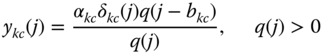
- The mean number of in‐service calls of service‐class k accepted in the system with
 ,
,  , via ( 2.16).
 - The mean number of in‐service calls of service‐class k accepted in the system with
 , via:
(2.43)
, via:
(2.43)
2.6 The Single‐Threshold Model under the BR Policy
2.6.1 The Service System
In the STM under the BR policy (STM/BR), ![]() b.u. are reserved to benefit calls of all other service‐classes apart from service‐class
b.u. are reserved to benefit calls of all other service‐classes apart from service‐class ![]() . The application of the BR policy in the STM is similar to that of the SRM/BR as the following example shows.
. The application of the BR policy in the STM is similar to that of the SRM/BR as the following example shows.
2.6.2 The Analytical Model
2.6.2.1 Steady State Probabilities
Similar to the SRM/BR, we adopt the Roberts method for the calculation of ![]() in the STM/BR.
in the STM/BR.
Based on the Roberts method, ( 2.38) takes the form [ 4]:

where  ,
,  ,
, ![]() ,
, ![]() is given by (1.65), and
is given by (1.65), and

2.6.2.2 CBP, Utilization, and Mean Number of In‐service Calls
Based on (2.44) and (2.45), we can determine the following performance measures:
- The CBP of service‐class
 calls with
  b.u.,
b.u.,  , via the formula [ 4]:
(2.46)where
, via the formula [ 4]:
(2.46)where
 is the normalization constant.
 - The CBP of service‐class k calls with
 b.u.,
b.u.,  , via (1.66).
 - The conditional CBP of service‐class k calls with
 given that
  ,
,  , via ( 2.40), while subtracting the BR parameter
  from
from  .
. - The link utilization,
 , via (1.54).
 - The mean number of service‐class k calls with
 b.u. in state
  ,
,  , via:
(2.47)
, via:
(2.47)

- The mean number of service‐class k calls with
 b.u. in state
  ,
,  , via:
(2.48)where
, via:
(2.48)where
 .
. - The mean number of in‐service calls of service‐class k accepted in the system with
 , via ( 2.16).
 - The mean number of in‐service calls of service‐class k accepted in the system with
 , via (2.43).
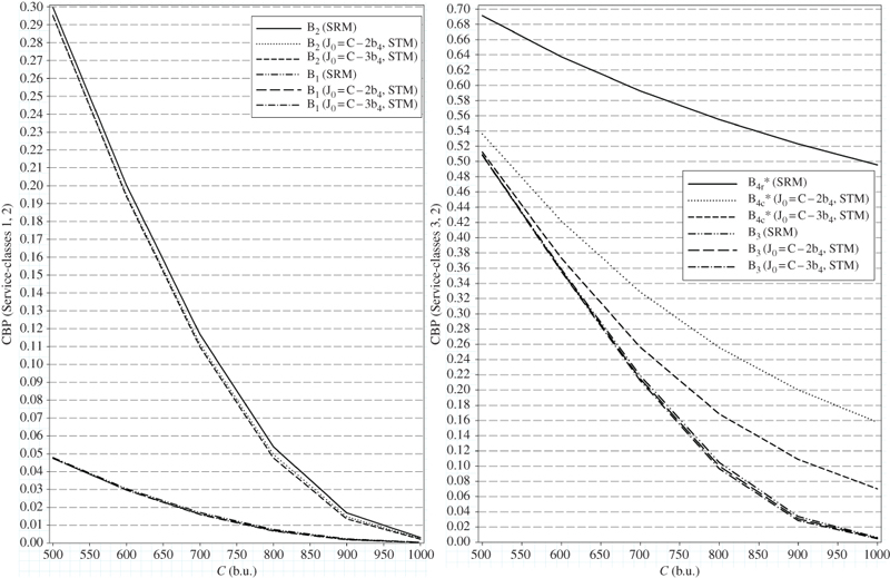
Figure 2.15 Left: CBP of service‐classes 1, 2 in the STM and SRM versus various values of  . Right: The corresponding graphs for service‐classes 3, 4 (Example 2.15).
Table 2.4 CBP of Example 2.15 (STM, ![]() or
or ![]() b.u., and
b.u., and ![]() ).
).
| CBP | Analytical results | Simulation results | Analytical results | Simulation results |
| 0.0474 | 0.0479 |
0.0003 | 0.00026 |
|
| 0.2953 | 0.2948 |
0.0025 | 0.0019 |
|
| 0.5086 | 0.5074 |
0.0054 | 0.0042 |
|
| 0.5361 | 0.5302 |
0.1579 | 0.1363 |
|
Table 2.5 CBP of Example 2.15 (STM, ![]() or
or ![]() b.u., and
b.u., and ![]() ).
).
| CBP | Analytical results | Simulation results | Analytical results | Simulation results |
| 0.0475 | 0.0480 |
0.0003 | 0.00017 |
|
| 0.2949 | 0.2948 |
0.0021 | 0.00137 |
|
| 0.5082 | 0.5074 |
0.0047 | 0.00297 |
|
| 0.5124 | 0.5113 |
0.0702 | 0.0511 |
|
Table 2.6 CBP of Example 2.15 (STM/BR, ![]() or
or ![]() b.u., and
b.u., and ![]() ).
).
| CBP | Analytical results | Simulation results | Analytical results | Simulation results |
| 0.3783 | 0.3799 |
0.00410 | 0.00332 |
|
| 0.3783 | 0.3799 |
0.00410 | 0.00333 |
|
| 0.3783 | 0.3799 |
0.00410 | 0.00332 |
|
| 0.3783 | 0.3799 |
0.00410 | 0.00333 |
|

Figure 2.16 CBP in the STM/BR and SRM/BR versus  and two values of
  (Example 2.15).
2.7 The Multi‐Threshold Model
2.7.1 The Service System
In the multi‐threshold model (MTM), there exist ![]() different thresholds which are common to all service‐classes [ 1, 2]. A call of service‐class
different thresholds which are common to all service‐classes [ 1, 2]. A call of service‐class ![]() with initial requirements
with initial requirements ![]() can use, depending on the occupied link bandwidth, one of the
can use, depending on the occupied link bandwidth, one of the ![]() requirements
requirements ![]() , where the pair
, where the pair ![]() is used when
is used when ![]() (where
(where ![]() . The maximum possible threshold is
. The maximum possible threshold is ![]() , while
, while ![]() . As far as the bandwidth requirements of a service‐class
. As far as the bandwidth requirements of a service‐class ![]() call are concerned, we assume that they decrease as
call are concerned, we assume that they decrease as ![]() increases, i.e.,
increases, i.e., ![]() , while by definition
, while by definition ![]() (see Figure 2.17).
(see Figure 2.17).

Figure 2.17 The MTM principle of operation.
2.7.2 The Analytical Model
2.7.2.1 Steady State Probabilities
To describe the MTM in steady state, the following LB equations are considered:

and

where ![]() denotes the mean number of service‐class
denotes the mean number of service‐class ![]() calls, with
calls, with ![]() , in state
, in state ![]() .
.
Similar to the analysis of the STM and based on (2.49) and (2.50), we have the following recursive formula for the calculation of ![]() [ 1, 2]:
[ 1, 2]:

where 
 and
and ![]() .
.
Note that in (2.51), ![]() expresses the upward migration approximation, while
expresses the upward migration approximation, while ![]() expresses the migration approximation.
expresses the migration approximation.
2.7.2.2 CBP, Utilization, and Mean Number of In‐service Calls
Based on ( 2.51), we can determine the following performance measures:
- The CBP of service‐class
 calls with
  b.u.,
b.u.,  , via the formula [ 2]:
(2.52)where
, via the formula [ 2]:
(2.52)where
 is the normalization constant.
 - The CBP of service‐class
 calls with
  b.u.,
b.u.,  , via (1.66).
 - The conditional CBP of service‐class
 calls with
  given that
 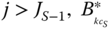 , via the formula:
(2.53)
, via the formula:
(2.53)
- The link utilization,
 , via (1.54).
 - The mean number of service‐class
 calls with
  b.u. in state
  , via:
(2.54)where
, via:
(2.54)where

- The mean number of service‐class
 calls with
  b.u. in state
  , via:
(2.55)where
, via:
(2.55)where
 .
. - The mean number of in‐service calls of service‐class
 accepted in the system with
  , via ( 2.16).
 - The mean number of in‐service calls of service‐class
 accepted in the system with
  , via:
(2.56)
, via:
(2.56)
2.8 The Multi‐Threshold Model under the BR Policy
2.8.1 The Service System
In the MTM under the BR policy (MTM/BR), ![]() b.u. are reserved to benefit calls of all other service‐classes apart from service‐class
b.u. are reserved to benefit calls of all other service‐classes apart from service‐class ![]() . The application of the BR policy in the MTM is similar to that of the MRM/BR.
. The application of the BR policy in the MTM is similar to that of the MRM/BR.
2.8.2 The Analytical Model
2.8.2.1 Steady State Probabilities
Similar to the MRM/BR, we adopt the Roberts method for the calculation of the unnormalized link occupancy distribution ![]() in the MTM/ BR.
in the MTM/ BR.
Based on the Roberts method, ( 2.51) takes the form [ 4]:

where 
 ,
, ![]() , and
, and

2.8.2.2 CBP, Utilization, and Mean Number of In‐service Calls
Based on (2.57) and (2.58), we can determine the following performance measures:
- The CBP of service‐class k calls with
 b.u.,
b.u.,  , via the formula [ 4]:
(2.59)where
, via the formula [ 4]:
(2.59)where
 is the normalization constant.
 - The CBP of service‐class
 calls with
  b.u.,
b.u.,  , via (1.66).
 - The conditional CBP of service‐class
 calls with
  given that
  , via the formula:
(2.60)
, via the formula:
(2.60)
- The link utilization,
 , via (1.54).
 - The mean number of service‐class
 calls with
  b.u. in state
  , via:
(2.61)where
, via:
(2.61)where

- The mean number of service‐class
 calls with
  b.u. in state
  , via:
(2.62)where
, via:
(2.62)where
 .
. - The mean number of in‐service calls of service‐class
 accepted in the system with
  , via ( 2.16).
 - The mean number of in‐service calls of service‐class
 accepted in the system with
  , via (2.56).

Figure 2.18 Left: CBP of service‐classes 1, 2, and 3 versus the sets of thresholds. Right: Conditional CBP of service‐class 4 versus the sets of thresholds (MTM) (Example 2.16).

Figure 2.19 Equalized CBP of all service‐classes versus the sets of thresholds (MTM/BR) (Example 2.16).
2.9 The Connection Dependent Threshold Model
2.9.1 The Service System
In the connection dependent threshold model (CDTM), bandwidth and service time requests depend on the total number ![]() of occupied b.u. of a link of capacity
of occupied b.u. of a link of capacity ![]() , as in the MTM. The only difference with the MTM is that different service‐classes may have different sets of thresholds. Specifically, we consider
, as in the MTM. The only difference with the MTM is that different service‐classes may have different sets of thresholds. Specifically, we consider ![]() service‐classes of Poisson arriving calls with mean arrival rates
service‐classes of Poisson arriving calls with mean arrival rates ![]() that require
that require ![]() b.u. per call and a mean service time
b.u. per call and a mean service time ![]() , exponentially distributed. Calls compete for the available bandwidth under the CS policy. The offered traffic‐load of calls of service‐class
, exponentially distributed. Calls compete for the available bandwidth under the CS policy. The offered traffic‐load of calls of service‐class ![]() is
is ![]() . Let
. Let ![]() , and
, and ![]() . Each arriving call of a service‐class
. Each arriving call of a service‐class ![]() may have
may have ![]() bandwidth and service‐time requirements, that is, one initial requirement with values
bandwidth and service‐time requirements, that is, one initial requirement with values ![]() and
and ![]() more requirements with values
more requirements with values ![]() , where
, where ![]() and
and ![]() , and
, and ![]() . The pair
. The pair ![]() is used when
is used when ![]() , where
, where ![]() and
and ![]() are two successive thresholds of service‐class
are two successive thresholds of service‐class ![]() , while
, while ![]() ; the highest possible threshold (other than
; the highest possible threshold (other than ![]() ) is
) is ![]() (see Figure 2.20). By convention,
(see Figure 2.20). By convention, ![]() and
and ![]() , while the pair
, while the pair ![]() is used when
is used when ![]() .
.

Figure 2.20 The CDTM principle of operation.
2.9.2 The Analytical Model
2.9.2.1 Steady State Probabilities
Similar to the MTM, the CDTM has no PFS. To describe the CDTM in steady state, the following LB equations are assumed:


where ![]() denotes the mean number of service‐class
denotes the mean number of service‐class ![]() calls, with
calls, with ![]() , in state
, in state ![]() .
.
Formulas (2.63) and (2.64) are graphically presented in Figure 2.22.
Similar to the analysis of the MTM and based on ( 2.63) and ( 2.64), we have the following recursive formula for the calculation of ![]() [ 4]:
[ 4]:

where 
 and
and ![]() .
.
As a summary, in order to derive (2.65), the following assumptions (approximations) are necessary:
- (i) The assumption that the LB equations ( 2.63) and ( 2.64) do exist. This is the first source of error in ( 2.65).
- (ii)
 is assumed negligible (i.e., zero) outside
  . This assumption is the migration approximation, and we name the state space in which
  , the migration space
  . Let us recall that in the migration space, calls accepted in the system with other than the maximum bandwidth requirement are negligible. This assumption is the second source of error in ( 2.65) and is represented by the variable
  .
. - (iii)
 is assumed negligible (i.e., zero), if
  and
and  . This is the upward migration approximation, and we name the state space in which
  , the upward migration space. Let us recall that in the upward migration space, calls accepted in the system with their maximum bandwidth are negligible. This assumption is the third source of error in ( 2.65) and is represented by the variable
  .
.
Note that in both (ii) and (iii), the values of ![]() and
and ![]() may not be negligible in the corresponding migration and upward migration spaces, respectively (see Example 2.18). The determination of these values can improve the accuracy of the CDTM, compared to simulation, but is beyond the scope of this book. The reader may refer to [7,8].
may not be negligible in the corresponding migration and upward migration spaces, respectively (see Example 2.18). The determination of these values can improve the accuracy of the CDTM, compared to simulation, but is beyond the scope of this book. The reader may refer to [7,8].

Figure 2.22 Graphical representation of the LB equations 2.63 (left) and 2.64 (right).

Figure 2.23 Migration and upward migration spaces (Example 2.18).
2.9.2.2 CBP, Utilization, and Mean Number of In‐service Calls
Based on ( 2.65), we can determine the following performance measures:
- The CBP of service‐class
 calls with
  b.u.,
b.u.,  , via:
(2.66)where
, via:
(2.66)where
 is the normalization constant.
 - The CBP of service‐class
 calls with
  b.u.,
b.u.,  , via (1.66).
 - The conditional CBP of service‐class
 calls with
  given that
  ,
,  , via:
(2.67)
, via:
(2.67)
- The link utilization,
 , via (1.54).
 - The mean number of service‐class
 calls with
  b.u. in state
  , via:
(2.68)where
, via:
(2.68)where

- The mean number of service‐class
 calls with
  b.u. in state
  ,
,  , via:
(2.69)
, via:
(2.69)
- The mean number of in‐service calls of service‐class
 accepted in the system with
  , via ( 2.16).
 - The mean number of in‐service calls of service‐class
 accepted in the system with
  , via ( 2.56).
2.10 The Connection Dependent Threshold Model under the BR Policy
2.10.1 The Service System
In the CDTM under the BR policy (CDTM/BR), ![]() b.u. are reserved to benefit calls of all other service‐classes apart from service‐class
b.u. are reserved to benefit calls of all other service‐classes apart from service‐class ![]() . The application of the BR policy in the CDTM is similar to that of the MTM/BR.
. The application of the BR policy in the CDTM is similar to that of the MTM/BR.
2.10.2 The Analytical Model
2.10.2.1 Link Occupancy Distribution
Similar to the MTM/BR, we adopt the Roberts method for the calculation of ![]() in the CDTM/BR. Based on the Roberts method, ( 2.65) takes the form [ 4]:
in the CDTM/BR. Based on the Roberts method, ( 2.65) takes the form [ 4]:

where 

 and
and ![]() .
.
2.10.2.2 CBP, Utilization, and Mean Number of In‐service Calls
Based on (2.70), we can determine the following performance measures:
- The CBP of service‐class k calls with
 b.u.,
b.u.,  , as follows [ 4]:
(2.71)where
, as follows [ 4]:
(2.71)where
 is the normalization constant.
 - The CBP of service‐class
 calls with
  b.u.,
b.u.,  , via (1.66).
 - The conditional CBP of service‐class
 calls with
  given that
  , via:
(2.72)
, via:
(2.72)
- The link utilization,
 , via (1.54).
 - The mean number of service‐class
 calls with
  b.u. in state
  , via:
(2.73)where
, via:
(2.73)where

- The mean number of service‐class
 calls with
  b.u. in state
  , via:
(2.74)where
, via:
(2.74)where
 .
. - The mean number of in‐service calls of service‐class
 accepted in the system with
  , via ( 2.16).
 - The mean number of in‐service calls of service‐class
 accepted in the system with
  , via ( 2.56).
2.11 Applications
We concentrate only on the CDTM since it comprises the retry and threshold models. The initial motivation for the CDTM was the available bit rate (ABR) service of asynchronous transfer mode (ATM) networks. The ABR service is a purely elastic service in which the notion of equivalent bandwidth is not well applicable (i.e., the ABR service cannot be considered a stream service having its average bandwidth per call, as constant rate). Therefore, a different model to the EMLM is needed, and this is the CDTM because it sufficiently models an elastic call at its set‐up phase (but not during the entire call duration) by adequately setting the threshold parameters. Thus, the CDTM is applicable to any elastic service at the call set‐up phase, as long as it is not a bandwidth hungry application wasting all the available bandwidth. For this reason, a threshold scheme must be applied (e.g., Figure 2.20). The logic behind the threshold scheme is that even if the available bandwidth of a link is large enough, a CAC does not always waste it on one call only, but saves a part of it for sharing with the next calls.
The minimum and the maximum bandwidth requirements of an elastic call are important CDTM parameters for the CBP calculation no matter what the thresholds are. The minimum bandwidth requirement is critical for the CBP value. If the minimum required bandwidth is zero, an elastic call should wait for any available bandwidth to start servicing. If the network (CAC) ignores the details of bandwidth requirements (i.e., the threshold scheme) of an elastic call, the assigned bandwidth will not meet the real needs of the call and the CBP calculation will not be accurate. Suppose, for instance, that an elastic call has the following thresholds scheme in a transmission link with bandwidth capacity of 19.2 Mbps: maximum rate of 1.536 Mbps for available link bandwidth at least 6.4 Mbps (first threshold at ![]() Mbps), rate of 768 kbps for available link bandwidth at least 3.2 Mbps at least (second threshold at
Mbps), rate of 768 kbps for available link bandwidth at least 3.2 Mbps at least (second threshold at ![]() Mbps), and minimum rate of 384 kbps for available link bandwidth less than 3.2 Mbps (third threshold at 19.2 Mbps, or at
Mbps), and minimum rate of 384 kbps for available link bandwidth less than 3.2 Mbps (third threshold at 19.2 Mbps, or at ![]() Mbps). Assume that the CAC knows only the minimum and maximum resource requirements of this elastic call, and offers to it (a) 700 kbps or (b) 1.536 Mbps when the available bandwidth is 4.0 Mbps at least in both cases. In the first case, the holding time will be estimated incorrectly (by taking into account 768 kbps instead of 700 kbps), while in the second case, although the holding time will be estimated correctly, the threshold scheme has been violated, therefore the CBP through the CDTM cannot be accurate. As far as the number of thresholds between the minimum and the maximum bandwidth requirements is concerned, several values exist since bandwidth is quantized and provided as a group of b.u. (trunks). So, in a realistic network environment the number of thresholds is manageable.
Mbps). Assume that the CAC knows only the minimum and maximum resource requirements of this elastic call, and offers to it (a) 700 kbps or (b) 1.536 Mbps when the available bandwidth is 4.0 Mbps at least in both cases. In the first case, the holding time will be estimated incorrectly (by taking into account 768 kbps instead of 700 kbps), while in the second case, although the holding time will be estimated correctly, the threshold scheme has been violated, therefore the CBP through the CDTM cannot be accurate. As far as the number of thresholds between the minimum and the maximum bandwidth requirements is concerned, several values exist since bandwidth is quantized and provided as a group of b.u. (trunks). So, in a realistic network environment the number of thresholds is manageable.
In what follows, we concentrate on the applicability of the CDTM to WCDMA networks. We have skipped straightforward applications, albeit some of them are very interesting, such as the application of the CDTM on smart grid, for a fine control of energy consumption [9].
Applicability of the CDTM to WCDMA Networks
The CDTM can be applied to WCDMA networks (in the uplink) in a similar way to the EMLM. A single BS controlling a cell can be modeled as a system of certain bandwidth capacity. The b.u. can be an equivalent bandwidth defined by the load factor introduced, for instance, by a lower rate service‐class (e.g., voice). The load factor is determined by the signal‐to‐noise ratio (SNR), data rate, and activity factor (probability that a call is active – transmits) of the associated service‐class. As far as the inter‐cell interference is concerned, it is assumed log‐normally distributed1 and independent of the cell load. A call is accepted for service as long as there are enough resources available in the cell. The CAC policy is based on the estimation of the increase in the total interference (intra‐ and inter‐cell interference plus thermal noise) caused by the acceptance of new calls. After call acceptance, the SNR of all in‐service calls deteriorates; because of this, WCDMA systems usually have no hard limits on call capacity. A call should not be accepted if it increases the noise of all in‐service calls above a tolerable level. Poisson arriving calls to a cell may have several contingency resource/QoS requirements.
Let us consider that the QoS offered to each service‐class ![]() belongs to one out of
belongs to one out of ![]() alternative QoS levels, which depend on the occupied cell resources. In what follows, a service‐class
alternative QoS levels, which depend on the occupied cell resources. In what follows, a service‐class ![]() call of QoS level
call of QoS level ![]() is referred to as service‐class
is referred to as service‐class ![]() call. A service‐class
call. A service‐class ![]() call is characterized by the following QoS parameters: (i)
call is characterized by the following QoS parameters: (i) ![]() , transmission bit rate, (ii)
, transmission bit rate, (ii) ![]() , mean service time (exponentially distributed), and (iii)
, mean service time (exponentially distributed), and (iii) ![]() , BER parameter.
, BER parameter.
The application of the CDTM for the call‐level performance evaluation of WCDMA networks is necessary when assuming that a WCDMA cell accommodates not only stream service‐classes but also elastic service‐classes, which are associated with individual sets of thresholds (indicating the occupied cell resources). A variation of an elastic service‐class is an adaptive service‐class, in which calls may reduce their resources/bandwidth, but their service time is kept fixed. We can therefore consider three types of service‐classes:
- Stream type: service‐classes that have only one QoS level (
 ).
). - Elastic type: service‐classes that have more than one QoS level (
 ) and the call's mean service time strongly depends on the QoS level (it holds:
  .
. - Adaptive type: service‐classes that have more than one QoS level (
 ) and the call's mean service time is the same for all QoS levels (it holds:
  .
.
Upon their arrival, elastic or adaptive calls select one resource requirement according to an associated threshold scheme; a resource requirement is not altered during the service‐time. For example, a QoS level can be assigned to an elastic service‐class ![]() call at the arrival time and is based on the occupied system resources (cell load
call at the arrival time and is based on the occupied system resources (cell load ![]() ), which is indicated through thresholds. The thresholds of an elastic service‐class
), which is indicated through thresholds. The thresholds of an elastic service‐class ![]() are denoted by
are denoted by ![]() . The QoS level assignment is performed as follows. If
. The QoS level assignment is performed as follows. If ![]() , then the elastic call is assigned the first QoS level
, then the elastic call is assigned the first QoS level ![]() and occupies
and occupies ![]() system resources for an exponentially distributed service time with mean
system resources for an exponentially distributed service time with mean ![]() . The symbol
. The symbol ![]() comes from the load factor (see 2.78). If
comes from the load factor (see 2.78). If ![]() , then the call is assigned to the second QoS level and occupies
, then the call is assigned to the second QoS level and occupies ![]() resources for an exponentially distributed service‐time with mean
resources for an exponentially distributed service‐time with mean ![]() , and so on. Finally, if
, and so on. Finally, if ![]() , then the call is assigned to the
, then the call is assigned to the ![]() QoS level and occupies
QoS level and occupies ![]() resources for an exponentially distributed service time with mean
resources for an exponentially distributed service time with mean ![]() . We assume that an elastic call has a certain amount of data to transmit. Therefore, a call's service time should be conversely proportional to the allocated resources. For this reason, the mean call service times,
. We assume that an elastic call has a certain amount of data to transmit. Therefore, a call's service time should be conversely proportional to the allocated resources. For this reason, the mean call service times, ![]() , are chosen so that the product
, are chosen so that the product ![]() remains constant for every QoS level
remains constant for every QoS level ![]() . As far as the offered traffic‐load of service‐class
. As far as the offered traffic‐load of service‐class ![]() calls is concerned, it is defined as
calls is concerned, it is defined as ![]() .
.
Interference and Call Admission Control
We assume perfect power control, i.e., at the BS, the same amount of power, ![]() , is received from each service‐class
, is received from each service‐class ![]() call. Since in WCDMA systems all users transmit within the same frequency band, a single user sees the signals generated by all other users as interference. Intra‐cell interference,
call. Since in WCDMA systems all users transmit within the same frequency band, a single user sees the signals generated by all other users as interference. Intra‐cell interference, ![]() , is caused by users of the cell and inter‐cell interference,
, is caused by users of the cell and inter‐cell interference, ![]() , is caused by users of the neighbouring cells. An amount of power
, is caused by users of the neighbouring cells. An amount of power ![]() is due to thermal noise in the cell and corresponds to the intra‐cell interference when the cell is empty.
is due to thermal noise in the cell and corresponds to the intra‐cell interference when the cell is empty.
The CAC is performed by measuring the noise rise, ![]() , which is defined as the ratio of the total received power at the BS,
, which is defined as the ratio of the total received power at the BS, ![]() , to the thermal noise power,
, to the thermal noise power, ![]() :
:

When a new call arrives, the CAC estimates the noise rise and if it exceeds a maximum value, ![]() , the new call is blocked and lost.
, the new call is blocked and lost.
Load factor and cell load
The cell load, ![]() , is defined as the ratio of the received power from all active users to the total received power:
, is defined as the ratio of the received power from all active users to the total received power:

From (2.75) and (2.76), the relation between the noise rise and the cell load is:
The maximum value of the cell load, ![]() , is the cell load which corresponds to the maximum noise rise,
, is the cell load which corresponds to the maximum noise rise, ![]() 2:
2: ![]() .
.
The resource/bandwidth requirement of a service‐class ![]() call is expressed by the load factor,
call is expressed by the load factor, ![]() [10]:
[10]:

where ![]() is the chip rate of the WCDMA carrier.
is the chip rate of the WCDMA carrier.
The cell load ![]() can be written as the sum of the intra‐cell load,
can be written as the sum of the intra‐cell load, ![]() (cell load derived from the active users of the reference cell), and the inter‐cell load,
(cell load derived from the active users of the reference cell), and the inter‐cell load, ![]() (cell load derived from the active users of the neighbouring cells), i.e.,
(cell load derived from the active users of the neighbouring cells), i.e., ![]() . The values of
. The values of ![]() and
and ![]() are given by 2.79 and 2.80, respectively:
are given by 2.79 and 2.80, respectively:

where ![]() is the number of active users of service‐class
is the number of active users of service‐class ![]() , while
, while

For a new service‐class ![]() call acceptance, the following condition must hold in the BS:
call acceptance, the following condition must hold in the BS:
That is, an arriving call with resource requirement ![]() is accepted in the cell if and only if, after its acceptance, the cell load remains below
is accepted in the cell if and only if, after its acceptance, the cell load remains below ![]() .
.
Local Blocking Probabilities
Due to (2.81), the probability that a new service‐class ![]() call is blocked when arriving at an instant with intra‐cell load,
call is blocked when arriving at an instant with intra‐cell load, ![]() , is called the local blocking probability (LBP),
, is called the local blocking probability (LBP), ![]() , and can be calculated by (based on ( 2.78)–( 2.80)):
, and can be calculated by (based on ( 2.78)–( 2.80)):
In ( 2.80), the ![]() can be modelled as a lognormal random variable (with parameters mean
can be modelled as a lognormal random variable (with parameters mean ![]() and variance
and variance ![]() ), which is independent of the intra‐cell interference. Hence, the mean,
), which is independent of the intra‐cell interference. Hence, the mean, ![]() , and the variance,
, and the variance, ![]() , of
, of ![]() are calculated by:
are calculated by:
Consequently, because of ( 2.80), the inter‐cell load, ![]() , will also be a lognormal random variable. Its mean,
, will also be a lognormal random variable. Its mean, ![]() , and variance,
, and variance, ![]() , are calculated as follows:
, are calculated as follows:

where the parameters ![]() and
and ![]() can be determined by solving (2.85) and (2.86):
can be determined by solving (2.85) and (2.86):

where ![]() is the coefficient of variation.
is the coefficient of variation.
Thus, (2.82) can be rewritten as:
The RHS of (2.89), is the cumulative distribution function (CDF) of ![]() . It is denoted by
. It is denoted by ![]() and can be calculated from:
and can be calculated from:

where ![]() is the well‐known error function.
is the well‐known error function.
Hence, if we substitute ![]() into (2.90), from ( 2.89) we can calculate the LBP of service‐class
into (2.90), from ( 2.89) we can calculate the LBP of service‐class ![]() calls as follows:
calls as follows:

Parameters' Discretization
To apply the CDTM in WCDMA systems, parameters' discretization is required. It is achieved by the introduction of a basic cell load unit ![]() (e.g., granularity of
(e.g., granularity of ![]() , used in Example 2.23). The CDTM parameters of system capacity, the total number of occupied b.u. in the system, the assigned number of b.u. to an in‐service call, and a bandwidth threshold are obtained by discretizing the cell load, the maximum cell load, the load factor, and the resource threshold, respectively:
, used in Example 2.23). The CDTM parameters of system capacity, the total number of occupied b.u. in the system, the assigned number of b.u. to an in‐service call, and a bandwidth threshold are obtained by discretizing the cell load, the maximum cell load, the load factor, and the resource threshold, respectively:

Incorporating the User Activity and LBP
The user activity is described by the activity factor, ![]() , which represents the fraction of the active period of a service‐class
, which represents the fraction of the active period of a service‐class ![]() call/user over the entire service time (
call/user over the entire service time (![]() ). In the CDTM, we consider that calls are active during the entire service time and we do not distinguish active users from passive users. However, in WCDMA systems it is essential to consider such a distinction because passive users do not consume any system resources. Hence, a system state
). In the CDTM, we consider that calls are active during the entire service time and we do not distinguish active users from passive users. However, in WCDMA systems it is essential to consider such a distinction because passive users do not consume any system resources. Hence, a system state ![]() does not represent the total number of occupied b.u. Instead, it represents the total number of b.u. that would be occupied if all (mobile) users were active. Let
does not represent the total number of occupied b.u. Instead, it represents the total number of b.u. that would be occupied if all (mobile) users were active. Let ![]() denote the total number of occupied b.u. at an instant. In the CDTM,
denote the total number of occupied b.u. at an instant. In the CDTM, ![]() is always equal to
is always equal to ![]() , while in WCDMA networks we have
, while in WCDMA networks we have ![]() . When all users are passive,
. When all users are passive, ![]() , while
, while ![]() when all users are active.
when all users are active.
The bandwidth occupancy, ![]() , is defined as the conditional probability that
, is defined as the conditional probability that ![]() b.u. are occupied in state
b.u. are occupied in state ![]() and, for user activity
and, for user activity ![]() , it can be calculated recursively by:
, it can be calculated recursively by:

where ![]() is the highest reachable system state,
is the highest reachable system state, ![]() for
for ![]() , and
, and ![]() is called resource/bandwidth share and denotes the proportion of the total occupied resources,
is called resource/bandwidth share and denotes the proportion of the total occupied resources, ![]() , from service‐class
, from service‐class ![]() calls (see (2.95)).
calls (see (2.95)).
In WCDMA systems, due to the intra‐/inter‐cell interference, blocking of a service‐class ![]() call may occur at any state
call may occur at any state ![]() with a probability
with a probability ![]() . This probability, called the local blocking factor (LBF), is calculated by summing over
. This probability, called the local blocking factor (LBF), is calculated by summing over ![]() the LBP multiplied by the corresponding bandwidth occupancies:
the LBP multiplied by the corresponding bandwidth occupancies:

where for ![]() use (2.91) with
use (2.91) with ![]() . Note that when
. Note that when ![]() ,
, ![]() (since in this case
(since in this case ![]() and
and ![]() ).
).
The service‐class ![]() bandwidth share in state
bandwidth share in state ![]() (requiring
(requiring ![]() b.u.) is derived assuming LB between adjacent systems states, while incorporating the LBF and the parameter delta (indicating the upward migration and migration approximations):
b.u.) is derived assuming LB between adjacent systems states, while incorporating the LBF and the parameter delta (indicating the upward migration and migration approximations):

where ![]() , while for
, while for ![]() :
:

State Probabilities and CBP
The state probabilities are given by:

for ![]() and
and ![]() for
for ![]() , with
, with ![]() .
.
The CBP of service‐class ![]() can be calculated by adding all the state probabilities multiplied by the corresponding LBFs:
can be calculated by adding all the state probabilities multiplied by the corresponding LBFs:

Due to the contingency bandwidth requirements, ![]() , we need also to sum over
, we need also to sum over ![]() in specific areas defined by thresholds. This is done with the aid of the parameter gamma:
in specific areas defined by thresholds. This is done with the aid of the parameter gamma:

2.12 Further Reading
Extensions of the retry or thresholds models are categorized in wired [11–18], wireless [19–21], and optical networks [22]. In [ 11], the threshold models are extended to include BPP traffic. The CBP calculations are based either on recursive formulas or on convolution algorithms. In [12] and [13], the single threshold of the STM is replaced by two thresholds. When a new call finds the occupied link bandwidth above a threshold, it can be accepted in the link with its lower bandwidth requirement (similar to the STM). When the occupied link bandwidth becomes less than the second threshold then an in‐service call (accepted with its lower bandwidth requirement) can increase its bandwidth to its peak‐bandwidth requirement. In [14] and [15], the CDTM is extended to allow call bandwidth compression/expansion of in‐service calls with [ 15] or without [ 14] the existence of the BR policy (more on the subject of bandwidth compression/expansion and Poisson arriving calls can be found in Chapters and ). In [16– 18], a variant of the SRM/STM is proposed. Specifically, some service‐classes are characterized cooperative and the rest non‐cooperative. Users from a cooperative service‐class can retry with a certain probability to be connected in the system with reduced bandwidth when blocked with their initial peak‐bandwidth and the total occupied bandwidth of the system is below a threshold. This behavior increases the QoS perceived by other users. In [ 19], the threshold models are extended to include the CBP calculation in the uplink of a UMTS network. To this end, the notion of local (soft) blocking is incorporated in the model. The latter means that a call may be blocked in any state of the system if its acceptance violates the QoS, in terms of noise, of all in‐service calls (see also [23–26]). In [20], the threshold models are extended for the call‐level analysis of the Iub interface in UMTS networks. In [ 21], a multi‐threshold teletraffic model for heterogeneous CDMA networks is proposed. The model enables QoS differentiation of handover traffic when elastic and adaptive service‐classes are present. Furthermore, an applicability framework is proposed that takes into account advances in Cloud‐RAN and self‐organizing network (SON) technologies. In [ 22], the CDTM is extended for the calculation of connection failure probabilities (due to unavailability of a wavelength) and CBP (due to the restricted bandwidth capacity of a wavelength) in hybrid TDM‐WDM PONs with DWA.
References
- 1 J. Kaufman, Blocking in a completely shared resource environment with state dependent resource and residency requirements. Proceedings of IEEE INFOCOM'92, Florence, Italy, 4–8 May 1992, pp. 2224–2232.
- 2 J. Kaufman, Blocking with retrials in a completely shared resource environment. North‐Holland, Performance Evaluation, 15(2):99–113, June 1992.
- 3 J. Kaufman, Blocking in a shared resource environment. IEEE Transactions on Communications, 29(10):1474–1481, October 1981.
- 4 I. Moscholios, M. Logothetis and G. Kokkinakis, Connection dependent threshold model: A generalization of the Erlang multiple rate loss model. Performance Evaluation, 48(1–4):177–200, May 2002.
- 5 I. Moscholios, M. Logothetis and T. Liokos, QoS equalization in the connection dependent threshold model. Proceedings of the Communication Systems, Networks and Digital Signal Processing Conference, CSNDSP 2002, Staffordshire, UK, 15–17 July 2002, pp. 442–445.
- 6 SIMSCRIPT III, http://www.simscript.com/.
- 7 M. Logothetis, I. Moscholios and G. Kokkinakis, Improvement of the connection dependent threshold model with the aid of reverse transition rates. 12th GI/ITG Conference on Measuring, Modelling and Evaluation of Computer and Comummunication Systems (MMB) and 3rd Polish‐German Teletraffic Symposium (PGTS), MMB&PGTS 2004, Dresden, Germany, 12–15 September 2004.
- 8 M. Logothetis, I. Moscholios and G. Kokkinakis, New connection dependent threshold model – A generalization of the Erlang multirate loss model. Mediterranean Journal of Electronics and Communications, 3(4):126–137, October 2007.
- 9 J. Vardakas, I. Zenginis, and M. Oikonomakou, Peak demand reduction through demand control: A mathematical analysis, Proceedings of the IEICE ICTF 2016, Patras, 6–8 July 2016.
- 10 V. Vassilakis, G. Kallos, I. Moscholios and M. Logothetis, An analytical model for elastic service‐classes in W‐CDMA networks, in Heterogenenous Networks, Vol. II ‐ Performance Analysis & Applications, D.SEA.6.1.6: Part of Final Deliverables of NoE Euro‐NGI to EC, River Publishers, pp. 277–299, 2009.
- 11 M. Glabowski, A. Kaliszan and M. Stasiak, Modeling product‐form state dependent systems with BPP traffic. Performance Evaluation, 67(3):174–197, March 2010.
- 12 M. Sobieraj, M. Stasiak, J. Weissenberg and P. Zwierzykowski, Analytical model fo the single threshold mechanism with hysteresis for multi‐service networks, IEICE Transactions on Communications, E95‐B(1):120–132, January 2012.
- 13 M. Sobieraj, M. Stasiak and P. Zwierzykowski, Model of the threshold mechanism with double hysteresis for multi‐service networks, in Computer Networks, CN 2012, A. Kwicien, P. Gaj and P. Stera (eds), Communications in Computer and Information Science, Vol. 291, Springer, Berlin, 2012.
- 14 V. Vassilakis, I. Moscholios and M. Logothetis, Call‐level performance modeling of elastic and adaptive service‐classes. Proceedings of the ICC, Glasgow, UK, June 2007.
- 15 V. Vassilakis, I. Moscholios and M. Logothetis, The extended connection‐dependent threshold model for call‐level performance analysis of multi‐rate loss systems under the bandwidth reservation policy. International Journal of Communication Systems, 25(7):849–873, July 2012.
- 16 S. Miyata, K. Yamaoka and H. Kinoshita, Optimal threshold characteristics of call admission control by considering cooperative behavior of users (loss model). Proceedings of the IEEE PACRIM, Victoria, Canada, August 2013.
- 17 S. Miyata, K. Yamaoka and H. Kinoshita, Optimal threshold configuration methods for flow admission control with cooperative users. IEICE Transactions on Communications, E97‐B(12):2706–2719, December 2014.
- 18 I. Moscholios, M. Logothetis and S. Shioda, Performance evaluation of multirate loss systems supporting cooperative users with a probabilistic behavior. IEICE Transactions on Communications, E100‐B(10):1778–1788, October 2017.
- 19 L. Popova and W. Koch, Analytical performance evaluation of mixed services with variable data rates for the uplink of UMTS. Proceedings of ISWCS'06, Valencia, Spain, September 2006.
- 20 D. Parniewicz, M. Stasiak, and P. Zwierzykowski, Multicast connections in mobile networks with embedded threshold mechanism, in Computer Networks, CN 2011, A. Kwicien, P. Gaj and P. Stera (eds), Communications in Computer and Information Science, Vol. 160, Springer, Berlin, 2011.
- 21 V. Vassilakis, I. Moscholios and M. Logothetis, Quality of service differentiation of elastic and adaptive services in CDMA networks: A mathematical modelling approach. Wireless Networks, 24(4):1279–1295, May 2018.
- 22 J. Vardakas, V. Vassilakis and M. Logothetis, Blocking analysis in hybrid TDM‐WDM PONs supporting elastic traffic. Proceedings of AICT, Athens, Greece, June 2008.
- 23 D. Staehle and A. Mäder, An analytic approximation of the uplink capacity in a UMTS network with heterogeneous traffic. Proceedings of the 18th International Teletraffic Congress, Berlin, September 2003.
- 24 V. Iversen, V. Benetis, N. Ha, and S. Stepanov, Evaluation of multi‐service CDMA networks with soft blocking. Proceedings of the ITC Specialist Seminar, pp. 223–227, Antwerp, August/September 2004.
- 25 V. Iversen, Evaluation of multi‐service CDMA networks with soft blocking. Proceedings of the 3rd Conference on Smart Spaces, ruSMART 2010, and 10th International Conference, NEW2AN 2010, St. Petersburg, Russia, August 2010.
- 26 I. Moscholios, G. Kallos, V. Vassilakis, M. Logothetis and M. Koukias, Congestion probabilities in W‐CDMA networks supporting calls of finite sources. Proceedings of HETNETs, Ilkley, West Yorkshire, UK, November 2013.