
12
Genomics
Genomics is the study of an organism’s genome or genetic material. In humans, genetic materials are stored in the form of Deoxyribonucleic Acid (DNA). These are the instructions that make up a human being, and 99.9% of the genomes in humans are identical and only 0.1% is different, which accounts for the differences in physical characteristics, such as eye color. Most of these variations are harmless, but some variants can cause health conditions, such as sickle cell anemia. Therefore, the analysis of such information can be used to predict or prevent a disease or provide personalized treatment, also known as precision medicine. There are four chemical bases present in DNA, namely adenine (A), thymine (T), cytosine (C), and guanine (G). They always bond in a particular manner; for example, adenine will always bond with thymine, and cytosine with guanine. The combination of these chemical bases is what makes up a DNA sequence.
Sequencing is at the heart of genomics. To understand what it means, the Human Genome Project (https://www.ncbi.nlm.nih.gov/pmc/articles/PMC6875757/pdf/arhw-19-3-190.pdf) was started in 1989 with the objective of sequencing one human genome within 15 years. This was completed in 12 years in 2001 and involved thousands of scientists. With the development of next-generation sequencing technology, the whole human genome can now be generated in about a day. A single human genome is around 3 billion base pairs long; a similar size has been seen for other organisms such as a mouse or a cow.
Since the time and cost of generating the genome sequence have significantly dropped, it has led to the generation of an enormous amount of data. So, in order to analyze this magnitude of data, we need powerful machines and a large amount of cost-effective storage. The good news is that DNA sequencing data is publicly available, and one of the largest repositories is the National Center for Biotechnology Information (NCBI). We can use statistical and machine learning (ML) models to gain insights from the genome data, which can be compute intensive. This poses two major challenges: big data and a massive ML model are required to make predictions, such as the prediction of promoters or predicting the masked DNA sequence.
Therefore, this chapter will help navigate these challenges by covering the following topics:
- Managing large genomics data on AWS
- Designing architecture for genomics
- Applying ML to genomics
Technical requirements
You should have the following prerequisites before getting started with this chapter:
- A web browser (for the best experience, it is recommended that you use a Chrome or Firefox browser)
- Access to the AWS account that you used in Chapter 5, Data Analysis
- Access to the SageMaker Studio development environment that we created in Chapter 5, Data Analysis
- Example Jupyter notebooks for this chapter are provided in the companion GitHub repository (https://github.com/PacktPublishing/Applied-Machine-Learning-and-High-Performance-Computing-on-AWS/tree/main/Chapter06)
Managing large genomics data on AWS
Apart from the large size of the genomics dataset, other challenges for managing it include discoverability, accessibility, availability, and storing it in a storage system that allows for scalable data processing while keeping the critical data safe. The responsible and secure sharing of genomic and health data is key to accelerating research and improving human health, is a stated objective of the Global Alliance for Genomics and Health (GA4GH). This approach requires two important things: one is a deep technical understanding of the domain, and the second is access to compute and storage resources. You can also find many genomics datasets hosted by AWS on the Registry of Open Data on AWS (https://registry.opendata.aws/).
Before you can begin any processing on the genomics dataset using cloud services, you need to make sure that it’s transferred and stored on the AWS cloud. For storing data, we recommend using Amazon Simple Storage Services (Amazon S3), as genomics data produced by next-generation sequencers are persisted in files, and a lot of genomic data analysis tools also take files as inputs and write the output back as files. For example, using an ML model for data analysis might involve taking large DNA sequence files as input and storing the inference or prediction results in a file, for which Amazon S3 makes a natural fit.
You can store genomics data securely by enabling server-side encryption with either Amazon S3-managed encryption keys (SSE-S3) or AWS Key Management Service (AWS KMS) keys. Moreover, Amazon S3 also allows you to enable the data life cycle by storing the infrequently accessed data in the Amazon S3 Standard-Infrequent Access (S3 Standard-IA) class tier or archiving the data to a low-cost storage option, such as Amazon S3 Glacier Deep Archive when the data is not in use to significantly reduce the cost. This pattern is discussed in detail in the Tiered storage for cost optimization section of Chapter 4, Data Storage.
For transferring genomics data to Amazon S3, you can use the AWS DataSync service, as discussed in Chapter 2, Data Management and Transfer.
Let’s take a closer look at the detailed architecture for applying ML models to the genomics dataset.
Designing architecture for genomics
In this section, we will describe a sample reference architecture for transferring, storing, processing, and gaining insights on genomics datasets on the AWS cloud, in a secure and cost-effective manner. Figure 12.1 shows a sample genomics data processing workflow:

Figure 12.1 – Genomics data processing workflow
Figure 12.1 shows the following workflow:
- A scientist or a lab technician will collect sample genomic data, for example, skin cells, prepare it in a lab, and then load it into a sequencer.
- The sequencer will then generate a sequence, which might be short DNA fragments. These are usually called reads because you are reading DNA.
- The DNA sequence is stored in an on-premises data storage system.
- The AWS DataSync service will then transfer the genomic data securely to the cloud; for further details, refer to Chapter 2, Data Management and Transfer.
- The raw genomic data is then stored on Amazon S3. You can use AWS Analytics tools for data processing.
- Amazon Genomics CLI is a purpose-built open source tool for processing raw genomics data in the cloud at a petabyte scale. For details, please refer to this link: https://aws.amazon.com/genomics-cli/.
- Optionally, we recommend storing the processed genomics data on Amazon Feature Store, which is a fully managed service for storing, sharing, versioning, and managing ML features for training and inference to enable the reuse of features across ML applications.
- You can add granular access control policies on genomics data stored on Amazon S3 or Amazon Feature Store by using the AWS Lake Formation service, based on your business requirements. For details on AWS Lake Formation, refer to this link: https://aws.amazon.com/lake-formation.
- Once the data is processed and stored on either Amazon Feature Store or Amazon S3, you can run ML models such as DNABERT (https://www.biorxiv.org/content/10.1101/2020.09.17.301879v1) using Amazon SageMaker to gain further insights or to predict the masked DNA sequence. The ML model can take a batch of genomic data, make inferences, and store the results back in Amazon S3.
- Additionally, you can archive the unused data to Amazon S3 Glacier Deep Archive to have significant cost savings on data storage.
Note
A detailed discussion on Amazon Genomics CLI, AWS Lake Formation, and Amazon Feature Store is out of scope for this chapter; however, we will use the DNABERT model in the Applying ML to genomics section of this chapter.
Let’s learn how to apply the ML model to genomics applications and predict masked sequences in a DNA sequence using a pretrained ML model.
Applying ML to genomics
Before we dive into ML model details, let’s first understand the genomic data, which is stored as DNA in every organism. There are four chemical bases present in DNA, namely Adenine (A), Thymine (T), Cytosine (C) and Guanine (G). They always bond in particular manner for example, Adenine will always bond with Thymine, and Cytosine with Guanine. The combination of these chemical bases is what makes up a DNA sequence, represented by the letters A, T, C, and G. A 20-length example of a DNA sequence is ACTCCACAGTACCTCCGAGA. A single complete sequence of the human genome is around 3 billion base pairs (bp) long and takes about 200 GB of data storage (https://www.science.org/doi/10.1126/science.abj6987).
However, for analyzing the DNA sequence, we don’t need the complete human genome sequence. Usually, we analyze a part of the human DNA; for example, to determine hair growth or skin growth, a lab technician will take a small section of human skin and prepare it to run through the next-generation sequencer, which will then read the DNA and generate the DNA sequence, which are short fragments of DNA. ML models can be used for various tasks, such as DNA classification, promoter recognition, interpretation of structural variation in human genomes, precision medicine, cancer research, and so on.
In this section, we will showcase how to fine-tune the DNABERT model using Amazon SageMaker for the proximal promoter recognition task. DNABERT is based on the BERT model fine-tuned on DNA sequences, as outlined in the research paper Supervised promoter recognition: a benchmark framework (https://bmcbioinformatics.biomedcentral.com/track/pdf/10.1186/s12859-022-04647-5.pdf). Therefore, let’s take an example of deploying a pretrained DNABERT model for promoter recognition using DNA sequence data on Amazon SageMaker service.
Amazon SageMaker is a fully managed service by AWS to assist ML practitioners in building, training, and deploying ML models. Although it provides features and an integrated development environment for each phase of ML, it is highly modular in nature, meaning if you already have a trained model, you can use the SageMaker hosting features to deploy the model for performing inference/predictions on your model. For details on the various types of deployment options provided by SageMaker, refer to Chapter 7, Deploying Machine Learning Models at Scale.
We will deploy a version of the DNABERT pretrained model provided by Hugging Face, an AI community with a library of 65K+ pretrained transformer models. Amazon SageMaker provides first-party deep learning containers for Hugging Face for both training and inference. These containers include Hugging Face pretrained transformer models, tokenizers, and dataset libraries. For a list of all the available containers, you can refer to this link: https://github.com/aws/deep-learning-containers/blob/master/available_images.md. These containers are regularly maintained and updated with security patches and remove undifferentiated heavy lifting for ML practitioners.
With a few lines of configuration code, you can deploy a pretrained model in the Hugging Face library on Amazon SageMaker, and start making predictions using your model. Amazon SageMaker provides a lot of features for deploying ML models. For example, in the case of real-time inference, when you choose to deploy the model as an API, set up an autoscaling policy to scale up and down the number of instances on which the model is deployed based on the number of invocations on the model. Additionally, you can do blue/green deployment, add security guardrails, auto-rollback, and so on, using Amazon SageMaker hosting features. For details on deploying models for inference, refer to this link: https://docs.aws.amazon.com/sagemaker/latest/dg/deploy-model.html. Now that we have understood the benefits of using Amazon SageMaker for deploying models and Hugging Face integration, let’s see how we can deploy a pretrained DNABERT model for promoter recognition.
Note
The full code for deploying the model is available on GitHub: https://github.com/PacktPublishing/Applied-Machine-Learning-and-High-Performance-Computing-on-AWS/blob/main/Chapter12/dnabert.ipynb.
We need to follow three steps for deploying pretrained transformer models for real-time inference provided by the Hugging Face library on Amazon SageMaker:
- Provide model hub configuration where we supply the Hugging Face model ID and the task – in our case, text classification.
- Create a HuggingFaceModel class provided by the SageMaker API, where we provide parameters such as the transformer version, PyTorch version, Python version, hub configuration, and role.
- Finally, we use the deploy() API, where we supply the number of instances and the type of instance on which to deploy the model.
The following code snippet showcases the three steps that we just outlined:
…
from sagemaker.huggingface import HuggingFaceModel
import sagemaker
role = sagemaker.get_execution_role()
# Step 1: Hub Model configuration. https://huggingface.co/models
hub = {
     'HF_MODEL_ID':'AidenH20/DNABERT-500down',
     'HF_TASK':'text-classification'
}
# Step 2: create Hugging Face Model Class
huggingface_model = HuggingFaceModel(
     transformers_version='4.17.0',
     pytorch_version='1.10.2',
     py_version='py38',
     env=hub,
     role=role,
)
# Step 3: deploy model to SageMaker Inference
predictor = huggingface_model.deploy(
     initial_instance_count=1, # number of instances
     instance_type='ml.m5.xlarge' # ec2 instance type
)
…
Using this code snippet, we basically tell SageMaker to deploy the Hugging Face model provided in 'HF_MODEL_ID' for the task mentioned in 'HF_TASK'; in our case, text classification, as we want to classify promoter regions by providing a DNA sequence. The HuggingFaceModel class defines the container on which the model will be deployed. Finally, the deploy() API launches the Hugging Face container defined by the HuggingFaceModel class and loads the model provided in the hub configuration to the initial number of instances and type of instances provided by the ML practitioner.
Note
The number of instances on which the model is deployed as an API can be updated even after the model is deployed.
Once the model is deployed, you can then use the predict() API provided by SageMaker to make inferences or predictions on the model, as shown in the following code snippet:
…
dna_sequence = 'CTAATC TAATCT AATCTA ATCTAG TCTAGT CTAGTA TAGTAA AGTAAT GTAATG TAATGC AATGCC ATGCCG TGCCGC GCCGCG CCGCGT CGCGTT GCGTTG CGTTGG GTTGGT TTGGTG TGGTGG GGTGGA GTGGAA TGGAAA GGAAAG GAAAGA AAAGAC AAGACA AGACAT GACATG ACATGA CATGAC ATGACA TGACAT GACATA ACATAC CATACC ATACCT TACCTC ACCTCA CCTCAA CTCAAA TCAAAC CAAACA AAACAG AACAGC ACAGCA CAGCAG AGCAGG GCAGGG CAGGGG AGGGGG GGGGGC GGGGCG GGGCGC GGCGCC GCGCCA CGCCAT GCCATG CCATGC CATGCG ATGCGC TGCGCC GCGCCA CGCCAA GCCAAG CCAAGC CAAGCC AAGCCC AGCCCG GCCCGC CCCGCA CCGCAG CGCAGA GCAGAG CAGAGG AGAGGG GAGGGT AGGGTT GGGTTG GGTTGT GTTGTC TTGTCC TGTCCA GTCCAA TCCAAC CCAACT CAACTC AACTCC ACTCCT CTCCTA TCCTAT CCTATT CTATTC TATTCC ATTCCT'
predictor.predict({
     'inputs': dna_sequence
})
…
The output will be the label with the highest probability. In our case, it’s either LABEL_0 or LABEL_1, denoting the absence or presence of a promoter region in a DNA sequence.
Note
The preceding code deploys the model as an API on a long-running instance, so if you are not using the endpoint, please make sure to delete it; otherwise, you will be charged for it.
You can also see the endpoint details on SageMaker Studio by clicking on an orange triangle icon (SageMaker resources) in the left navigation panel and selecting Endpoints, as shown in the following screenshot:

Figure 12.2 – Accessing Endpoints on SageMaker Studio
This will show all the SageMaker endpoints (models deployed for real-time inference as an API). Double-clicking on the endpoint name will show you the details by calling the DescribeEndpoint() API behind the scenes. The SageMaker Studio UI shows you a lot of options, such as Test inference, Data quality, Model quality, Model explainability, Model bias, Monitoring job history, and AWS settings. The data is populated on these tabs based on the features you have enabled; for example, to understand the data and model quality, you need to enable the model monitoring feature of SageMaker, which monitors the models deployed as real-time endpoints on a schedule set by you, compares it with baseline statistics, and stores the report in S3. For details on model monitoring, refer to this link: https://docs.aws.amazon.com/sagemaker/latest/dg/model-monitor.html.
The AWS settings tab, on the other hand, will always be populated with model endpoint metadata, such as the endpoint name, type, status, creation time, last updated time, Amazon Resource Name (ARN), endpoint runtime settings, endpoint configuration settings, production variants (in case you have more than one variant of the same model), instance details (type and number of instances), model name, and lineage, as applicable. Figure 12.3 shows some of the metadata associated with the endpoint:
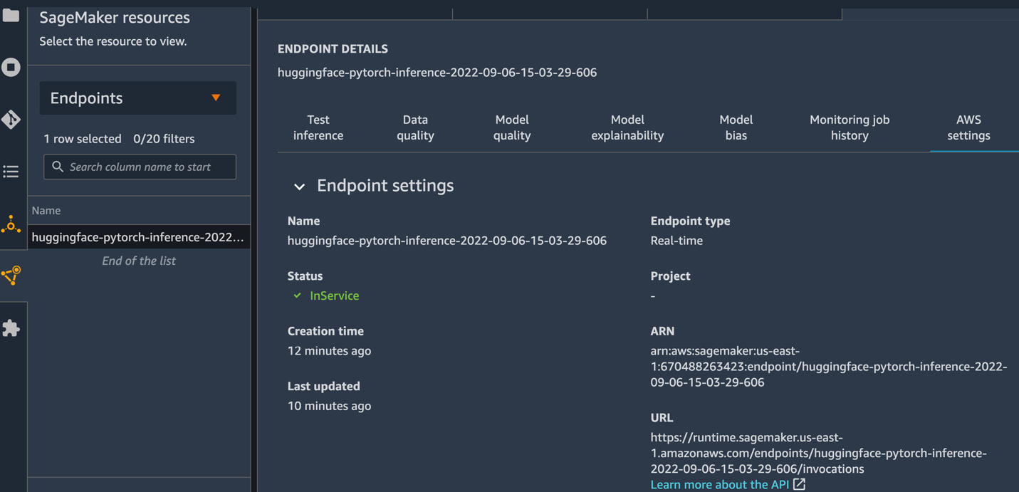
Figure 12.3 – SageMaker endpoint details
Also, if you quickly want to test your model from the SageMaker Studio UI, you can click on Test inference, provide a payload (input request) in JSON format in JSON editor, as shown in Figure 12.4, and quickly see the response provided by the model:
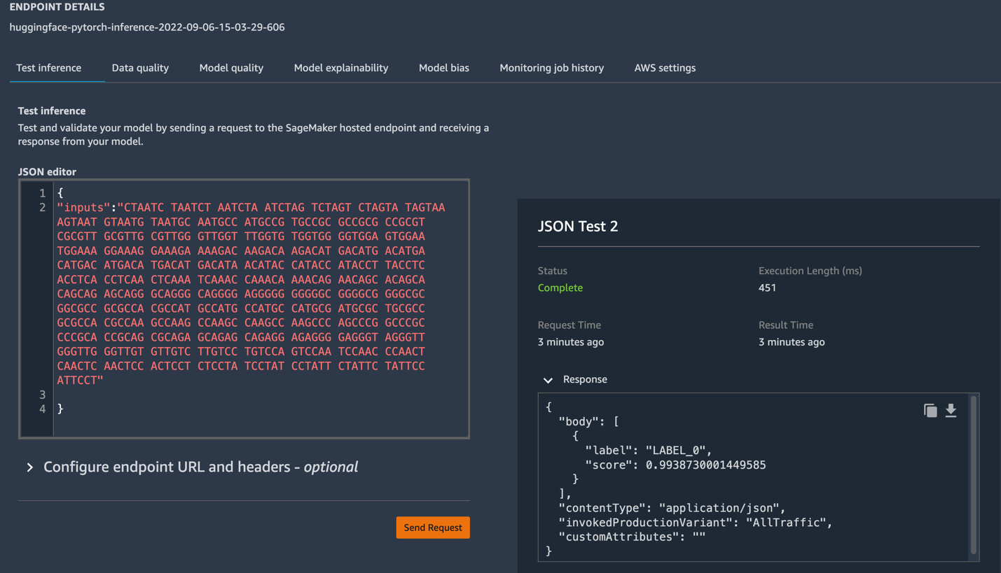
Figure 12.4 – Test inference from the SageMaker Studio UI
Now that we understand how pretrained models on the Hugging Face model library can be deployed and tested on Amazon SageMaker, let’s take another example of how to fine-tune the pretrained model in the Hugging Face library, and deploy the fine-tuned model. For this section, we will use a BERT-based model trained on protein sequences known as ProtBERT, published in this research paper: https://www.biorxiv.org/content/10.1101/2020.07.12.199554v3.
The study of protein structure, functions, and interactions is called proteomics, which takes the help of genomic studies as proteins are the functional product of the genome. Both proteomics and genomics are used to prevent diseases and are an active part of drug discovery. Although there are a lot of tasks that contribute to drug discovery, protein classification, and secondary structure identification play a vital role. In the following section, we will understand how to fine-tune a large protein model (the Hugging Face library) to predict the secondary structure of a protein using the distributed training features of Amazon SageMaker.
Protein secondary structure prediction for protein sequences
Protein sequences are made up of 20 essential amino acids, each represented by a capital letter. They combine to form a protein sequence, which you can use to do protein classification or predict the secondary structure of the protein, among other tasks. Protein sequences assume a particular 3D structure based on constraints, which are optimized for undertaking a particular function. You can think of these constraints as rules of grammar or meaning in natural language, which allows us to use natural language processing (NLP) techniques to protein sequences.
In this section, we will focus on fine-tuning the prot_t5_xl_uniref50 model, which has around 11 billion parameters, and you can use the same training script to fine-tune a smaller prot_bert_bfd model, which has close to 420 million parameters, with different configuration to accommodate the size of the model. The code for fine-tuning the prot_t5_xl_uniref50 model is provided in the GitHub repository: https://github.com/PacktPublishing/Applied-Machine-Learning-and-High-Performance-Computing-on-AWS/tree/main/Chapter12.
To create a SageMaker training job using the model in the Hugging Face library, we will need a Hugging Face estimator from SageMaker SDK. The estimator class will handle all the training tasks based on the configuration that we provide. For example, to train a Hugging Face model with the basic configuration, we will need to provide the following parameters:
- entry_point: This is where we will specify the training script for training the model.
- source_dir: This is the name of the folder where the training script or other helper files will reside.
- instance_type: This is the type of machine in the cloud where the training script will run.
- instance_count: This is the number of machines in the cloud that will be launched for running the training job. If the count is greater than 1, then it will automatically launch a cluster.
- transfomer_version, pytorch_version, py_version: These determine the version of transformers, PyTorch, and Python that will be present in the container. Based on the value of these parameters, SageMaker will fetch the appropriate container, which will be provisioned onto the instances (machines) in the cloud.
- hyperparameters: This defines the named arguments that will be passed to the training script.
The following code snippet formalizes these parameters into a SageMaker training job:
...
huggingface_estimator = HuggingFace(entry_point='train.py',
                           source_dir='./code',
                           instance_type='ml.g5.12xlarge',
                           instance_count=1,
                           role=role,
                           transformers_version='4.12',
                           pytorch_version='1.9',
                           py_version='py38',
                           hyperparameters=hyperparameters)
...
Once the estimator is defined, you can then provide the S3 location (path) of your data to start the training job. SageMaker provides some very useful environment variables for a training job, which include the following:
- SM_MODEL_DIR: This provides the path where the training job will store the model artifacts, and once the job finishes, the stored model in this folder is directly uploaded to the S3 output location.
- SM_NUM_GPUS: This represents the number of GPUs available to the host.
- SM_CHANNEL_XXXX: This represents the input data path for the specified channel. For example, data, in our case, will correspond to the SM_CHANNEL_DATA environment variable, which is used by the training script, as shown in the following code snippet:
…
# starting the train job with our uploaded datasets as input
huggingface_estimator.fit({'data': data_input_path})…
When we call the fit() method on the Hugging Face estimator, SageMaker will first provision the ephemeral compute environment, and copy the training script and data to the compute environment. It will then kick off the training, save the trained model to the S3 output location provided in the estimator class, and finally, tear down all the resources so that users only pay for the amount of time the training job was running for.
Note
For more information on the SageMaker Hugging Face estimator, as well as how to leverage the SageMaker SDK to instantiate the estimator, please see the AWS documentation (https://docs.aws.amazon.com/sagemaker/latest/dg/hugging-face.html), and the SageMaker SDK documentation (https://sagemaker.readthedocs.io/en/stable/frameworks/huggingface/sagemaker.huggingface.html#hugging-face-estimator).
We will extend this basic configuration to fine-tune prot_t5_xl_uniref50 with 11 billion parameters using the distributed training features of SageMaker.
Before we do a deeper dive into the code, let’s first understand some of the concepts that we will leverage for training the model. Since it’s a big model, the first step is to get an idea of the size of the model, which will help us determine whether it will fit in a single GPU memory or not. The SageMaker model parallel documentation (https://docs.aws.amazon.com/sagemaker/latest/dg/model-parallel-intro.html) gives a good idea of estimating the size of the model. For a training job that uses automatic mixed precision (AMP) with a floating-point 16-bit (FP16) size, using Adam optimizers, we can calculate the memory required per parameter using the following breakdown, which comes to about 20 bytes:
- An FP16 parameter ~ 16 bits or 2 bytes
- An FP16 gradient ~ 16 bits or 2 bytes
- An FP32 optimizer state ~ 64 bits or 8 bytes based on the Adam optimizers
- An FP32 copy of parameter ~ 32 bits or 4 bytes (needed for the optimizer apply (OA) operation)
- An FP32 copy of gradient ~ 32 bits or 4 bytes (needed for the OA operation)
Therefore, our model with 11 billion parameters will require more than 220 GB of memory, which is larger than the typical GPU memory currently available on a single GPU. Even if we are able to get such a machine with GPU memory greater than 220 GB, it will not be cost-effective, and we won’t be able to scale our training job. Another constraint to understand here is the batch size, as we will need at least one batch of data in the memory to begin training. Using a smaller batch size will drive down the GPU utilization and degrade the training efficiency, as the model might not be able to converge.
Hence, we will have to partition our model into multiple GPUs, and in order to increase the batch size, we will also need to shard the data. So, we will use a hybrid approach that will utilize both data parallel and model parallel approaches. This approach has been explained in detail in Chapter 6, Distributed Training of Machine Learning Models.
Since our model size is 220 GB, we will have to use a mechanism in the training job, which will optimize it for memory in order to avoid out of memory (OOM) errors. For memory optimization, the SageMaker model parallel library provides two types of model parallelism, namely, pipeline parallelism and tensor parallelism, along with memory-saving techniques, such as activation checkpointing, activation offloading, and optimizer state sharding. Let’s understand each of these terms:
- Pipeline parallelism: This means partitioning the model into different GPUs. This goes as a parameter to the training job, and based on the parallelism degree provided, the library will create different partitions. For example, we are training the model with 4 GPUs, and if the partitions parameter value provided in the configuration is 2, then the model will be divided into 2 partitions across 4 GPUs, meaning it will have 2 model replicas. Since, in this case, the number of GPUs is greater than the number of partitions, we will have to enable distributed data parallel by setting the ddp parameter to true. Otherwise, the training job will give an error. Pipeline parallelism with ddp enabled is illustrated in Figure 12.5:

Figure 12.5 – Showcasing the hybrid approach with model and data parallelism
- Tensor Parallelism: This applies the same concept as pipeline parallelism and goes a step further to divide the largest layer of our model and places it on different nodes. This concept is illustrated in Figure 12.6:

Figure 12.6 – Tensor parallelism shards tensors (layers) of the model across GPUs
- Activation checkpointing: This helps in reducing memory usage by clearing out the activations of layers and computing it again during the backward pass. For any deep learning model, the data is first passed through the intermediary layers in the forward pass, which compute the outputs, also known as activations. These activations need to be stored as they are used for computing gradients during the backward pass. Now, storing activations for a large model in memory can increase memory usage significantly and can cause bottlenecks. In order to overcome this issue, an activation checkpointing or gradient checkpointing technique comes in handy, which clears out the activations of intermediary layers.
Note
Activation checkpointing results in extra computation time in order to reduce memory usage.
- Activation offloading: This uses activation checkpointing, where it only keeps a few activations in the GPU memory during the model training. It offloads the checkpointed activations to CPU memory during the forward pass, which are loaded back to the GPU during the backward pass of a particular micro-batch of data.
- Optimizer state sharding: This is another useful memory-saving technique that partitions the state of the optimizers described by the set of weights across the data parallel device groups. It can be used only when we are using a stateful optimizer, such as Adam or FP16.
Note
Since optimizer state sharding partitions the optimizer state across the data parallel device groups, it will only become useful if the data parallel degree is greater than one.
Another important concept to understand with model parallelism is the micro-batch, which is a smaller subset of the batch of data. During training, you pass a certain number of records of data forward and backward through the layers, known as a batch or sometimes a mini-batch. A full pass through your dataset is called an epoch. SageMaker model parallelism shards the batch into smaller subsets, which are called micro-batches. These micro-batches are then passed through the pipeline scheduler to increase GPU utilization. The pipeline scheduler is explained in detail in Chapter 6, Distributed Training of Machine Learning Models.
So, now that we understand the memory-saving techniques used by the SageMaker model parallel library let’s see how we can use them in the code. The following code snippet wraps all the memory-saving techniques together in a simple manner:
…
# configuration for running training on smdistributed Model Parallel
mpi_options = {
    "enabled": True,
    "processes_per_host": 8,
}
smp_options = {
    "enabled":True,
    "parameters": {
        "microbatches": 1,
        "placement_strategy": "cluster",
        "pipeline": "interleaved",
        "optimize": "memory",
        "partitions": 4,
        "ddp": True,
        # "tensor_parallel_degree": 2,
        "shard_optimizer_state": True,
        "activation_checkpointing": True,
        "activation_strategy": "each",
        "activation_offloading": True,
    }
}
distribution = {
    "smdistributed": {"modelparallel": smp_options},
    "mpi": mpi_options
}
…
All the memory-saving techniques are highlighted in the code snippet, where you first have to make sure to set the optimize parameter to memory. This instructs the SageMaker model splitting algorithm to optimize for memory consumption. Once this is set, then you can simply enable other memory-saving features by setting their value to true.
You will then supply the distribution configuration to the HuggingFace estimator class, as shown in the following code snippet:
…
huggingface_estimator = HuggingFace(entry_point='train.py',
                           source_dir='./code',
                           instance_type='ml.g5.48xlarge',
                           instance_count=1,
                           role=role,
                           transformers_version='4.12',
                           pytorch_version='1.9',
                           py_version='py38',
                           distribution= distribution,
                           hyperparameters=hyperparameters)
huggingface_estimator.fit({'data': data_input_path})
…
As you can see, we also provide the train.py training script as entry_point to the estimator. In Chapter 6, Distributed Training of Machine Learning Models, we understood that when we are using model parallel, we have to update our training script with SageMaker model parallel constructs. In this example, since we are using the HuggingFace estimator and the Trainer API for model training, it has built-in support for SageMaker model parallel. So, we simply import the Hugging Face Trainer API and provide configuration related to model training, and based on the model parallel configuration provided in the HuggingFace estimator, it will invoke the SageMaker model parallel constructs during model training.
In our train.py script, first, we need to import the Trainer module, as shown in the following code snippet:
…
from transformers.sagemaker import SageMakerTrainingArguments as TrainingArguments
from transformers.sagemaker import SageMakerTrainer as Trainer
…
Since we are training a T5-based BERT model (prot_t5_xl_uniref50) we will also need to import the T5Tokenizer and T5ForConditionalGeneration modules from the transformers library:
…
from transformers import AutoTokenizer, T5ForConditionalGeneration, AutoModelForTokenClassification, BertTokenizerFast, EvalPrediction, T5Tokenizer
…
The next step is to transform the protein sequences and load them into a PyTorch DataLoader. After we have the data in DataLoader, we will provide TrainingArguments, as shown in the following code snippet, which will be used by the Trainer API:
…
training_args = TrainingArguments(
    output_dir='./results',         # output directory
    num_train_epochs=2,              # total number of training epochs
    per_device_train_batch_size=1,   # batch size per device during training
    per_device_eval_batch_size=1,   # batch size for evaluation
    warmup_steps=200,                # number of warmup steps for learning rate scheduler
    learning_rate=3e-05,             # learning rate
    weight_decay=0.0,                # strength of weight decay
    logging_dir='./logs',            # directory for storing logs
    logging_steps=200,               # How often to print logs
    do_train=True,                   # Perform training
    do_eval=True,                    # Perform evaluation
    evaluation_strategy="epoch",     # evalute after each epoch
    gradient_accumulation_steps=32,  # total number of steps before back propagation
    fp16=True,                       # Use mixed precision
    fp16_opt_level="02",             # mixed precision mode
    run_name="ProBert-T5-XL",      # experiment name
    seed=3,                         # Seed for experiment reproducibility
    load_best_model_at_end=True,
    metric_for_best_model="eval_accuracy",
    greater_is_better=True,
    save_strategy="epoch",
    max_grad_norm=0,
    dataloader_drop_last=True,
    )
…
As you can see, TrainingArguments contains a list of hyperparameters, such as the number of epochs, learning rate, weight decay, evaluation strategy, and so on, which will be used for model training. For details on the different hyperparameters for the TrainingArguments API, you can refer to this URL: https://huggingface.co/docs/transformers/v4.24.0/en/main_classes/trainer#transformers.TrainingArguments. Make sure that when you are providing TrainingArguments, the value of dataloader_drop_last is set to true. This will make sure that the batch size is divisible by the micro-batches, and setting fp16 to true will use the automatic mixed precision for model training, which also helps reduce the memory footprint, as floating-point 16 takes 2 bytes to store a parameter.
Now, we will define the Trainer API, which takes TrainingArguments and the training and validation datasets as input:
…
trainer = Trainer(
    model_init=model_init,                # the instantiated Transformers model to be trained
    args=training_args,                   # training arguments, defined above
    train_dataset=train_dataset,          # training dataset
    eval_dataset=val_dataset,             # evaluation dataset
    compute_metrics = compute_metrics,    # evaluation metrics
    )
…
Once the Trainer API has been defined, the model training is kicked off with the train() method, and once the training is complete, we will use the save_model() method to save the trained model to the specified model directory:
…
trainer.train()
trainer.save_model(args.model_dir)
…
The save_model() API takes the model path as a parameter, coming from the SM_MODEL_DIR SageMaker container environment variable and parsed as a model_dir variable. The model artifacts stored in this path will then be copied to the S3 path specified in the HuggingFace estimator, and all the resources, such as the training instance, will then be torn down so that users only pay for the duration of the training job.
Note
We are training a very large model, prot_t5_xl_uniref50, with 11 billion parameters on a very big instance, ml.g5.48xlarge, which is an NVIDIA A10G tensor core machine with 8 GPUs and 768 GB of GPU memory. Although we are using model parallel, the training of the model will take more than 10 hours, and you will incur a cost for it. Alternatively, you can use a smaller model, such as prot_bert_bfd, which has approximately 420 million parameters and is pretrained on protein sequences. Since it’s a relatively smaller model that can fit into a single GPU memory, you can only use the SageMaker distributed data parallel library, as described in Chapter 6, Distributed Training of Machine Learning Models.
Once the model is trained, you can deploy the model using the SageMaker HuggingFaceModel class, as explained in the Applying ML to genomics main section of this chapter, or simply use the huggingface_estimator.deploy() API, as shown in the following code snippet:
…
predictor = huggingface_estimator.deploy(1,"ml.g4dn.xlarge")
…
Once the model is deployed, you can use the predictor variable to make predictions:
…
predictor.predict(input_sequence)
…
Note
Both the discussed deployment options will deploy the model for real-time inference as an API on a long-running instance. So, if you are not using the endpoint, make sure to delete it; otherwise, you will incur a cost for it.
Now that we understand the applications of ML to genomics, let’s recap what we have learned so far in the next section.
Summary
In this chapter, we started with understanding the concepts of genomics and how you can store and manage large genomics data on AWS. We also discussed the end-to-end architecture design for transferring, storing, analyzing, and applying ML to genomics data using AWS services. We then focused on how you can deploy large state-of-the-art models for genomics, such as DNABERT, for promoter recognition tasks using Amazon SageMaker with a few lines of code and how you can test your endpoint using code and the SageMaker Studio UI.
We then moved on to understanding proteomics, which is the study of protein sequences, structure, and their functions. We walked through an example of predicting protein secondary structure for protein sequences using a Hugging Face pretrained model with 11 billion parameters. Since it is a large model with memory requirements greater than 220 GB, we explored various memory-saving techniques, such as activation checkpointing, activation offloading, optimizer state sharding, and tensor parallelism, provided by the SageMaker model parallel library. We then used these techniques to train our model for predicting protein structure. We also understood how SageMaker provides integration with Hugging Face and makes it simple to use state-of-the-art models, which otherwise need a lot of heavy lifting in order to train.
In the next chapter, we will review another domain, autonomous vehicles, and understand how high-performance computing capabilities provided by AWS can be used for training and deploying ML models at scale.