5

Data Analysis

One of the fundamental principles behind any large-scale data science procedure is the simple fact that any Machine Learning (ML) model produced is only as good as the data on which it is trained. Beginner data scientists often make the mistake of assuming that they just need to find the right ML model for their use case and then simply train or fit the data to the model. However, nothing could be further from the truth. Getting the best possible model requires exploring the data, with the goal being to fully understand the data. Once the data scientist understands the data and how the ML model can be trained on it, the data scientist often spends most of their time further cleaning and modifying the data, also referred to as wrangling the data, to prepare it for model training and building.

While this data analysis task may seem conceptually straightforward, the task becomes far more complicated when we factor in the type (images, text, tabular, and so on) and the amount/volume of data we are exploring. Furthermore, where the data is stored and getting access to it can also make the exercise even more overwhelming for the data scientist. For example, useful ML data may be stored within a data warehouse or located within various relational databases, often requiring various tools or programmatic API calls to mine the right data. Likewise, key information may be located across multiple file servers or within various buckets of a cloud-based object store. Locating the data and ensuring the correct permissions to access the data can further delay a data scientist from getting started.

So, with these challenges in mind, in this chapter, we will review some practical ways to explore, understand, and essentially wrangle different types, as well as large quantities of data, to train ML models. Additionally, we will examine some of the capabilities and services that AWS provides to make this task less daunting.

Therefore, this chapter will cover the following topics:

• Exploring data analysis methods
• Reviewing AWS services for data analysis
• Analyzing large amounts of structured and unstructured data
• Processing data at scale on AWS

Technical requirements

You should have the following prerequisites before getting started with this chapter:

• Familiarity with AWS services and their basic usage.
• A web browser (for the best experience, it is recommended that you use a Chrome or Firefox browser).
• An AWS account (if you are unfamiliar with how to get started with an AWS account, you can go to this link: https://aws.amazon.com/getting-started/).
• Familiarity with the AWS Free Tier (the Free Tier will allow you to access some of the AWS services for free, depending on resource limits. You can familiarize yourself with these limits at this link: https://aws.amazon.com/free/).
• Example Jupyter notebooks for this chapter are provided in the companion GitHub repository (https://github.com/PacktPublishing/Applied-Machine-Learning-and-High-Performance-Computing-on-AWS/tree/main/Chapter05).

Exploring data analysis methods

As highlighted at the outset of this chapter, the task of gathering and exploring these various sources of data can seem somewhat daunting. So, you may be wondering at this point where and how to begin the data analysis process? To answer this question, let’s explore some of the methods we can use to analyze your data and prepare it for the ML task.

Gathering the data

One of the first steps to getting started with a data analysis task is to gather the relevant data from various silos into a specific location. This single location is commonly referred to as a data lake. Once the relevant data has been co-located into a single data lake, the activity of moving data in or out of the lake becomes significantly easier.

For example, let’s imagine for a moment that a data scientist is tasked with building a product recommendation model. Using the data lake as a central store, they can query a customer database to get all the customer-specific data, typically from a relational database or a data warehouse, and then combine the customer’s clickstream data from the web application’s transaction logs to get a common source of all the required information to predict product recommendations. Moreover, by sourcing product-specific image data from the product catalog, the data scientist can further explore the various characteristics of product images that may enhance or contribute to the ML model’s predictive potential.

So, once that holistic dataset is gathered together and stored in a common repository or data store, we can move on to the next approach to data analysis, which is understanding the data structure.

Understanding the data structure

Once the data has been gathered into a common location, before a data scientist can fully investigate how it can be used to suggest an ML hypothesis, we need to understand the structure of the data. Since the dataset may be created from multiple sources, understanding the structure of the data is important before it can be analyzed effectively.

For instance, if we continue with the product recommendation example, the data scientist may work with structured customer data in the form of a tabular dataset from a relational database or data warehouse. Added to this, when pulling the customer interaction data from the web servers, the data scientist may work with time series or JSON formatted data, commonly referred to as semi-structured data. Lastly, when incorporating product images into the mix, the data scientist will deal with image data, which is an example of unstructured data.

So, understanding the nature or structure of the data determines how to extract the critical information we need and analyze it effectively. Moreover, knowing the type of data we’re dealing with will also influence the type of tools, such as Application Programming Interfaces (APIs), and even the infrastructure resources required to understand data.

Note

We will be exploring these tools and infrastructure resources in depth further on in the chapter.

Once we understand the data structure, we can apply this understanding to another technique of data analysis, that is, describing the data itself.

Describing the data

Once we understand the data’s structure, we can describe or summarize the characteristics of the data to further explore how these characteristics influence our overall hypothesis. This methodology is commonly referred to as applying descriptive statistics to the data, whereby a data scientist will try to describe and understand the various features of the dataset by summarizing the collective properties of each feature within the data in terms of centrality, variability, and data counts.

Let’s explore what each of these terms means to see how they can be used to describe the data.

Determining central tendency

By using descriptive statistics to summarize the central tendency of the data, we are essentially focusing on the average, middle, or center position within the distribution of a specific feature of the dataset. This gives the data scientist an idea of what is normal or average about a feature of the dataset, allowing them to compare these averages with other features of the data or even the entirety of the data.

For example, let’s say that customer A visited our website 10 times a day but only purchased 1 item. By comparing the average visits of customer A with the total number of customer visits, we can see how customer A ranks in comparison. If we then compare the number of items purchased with the total number of items, we can further gauge what is considered normal based on the customer’s ranking.

Measuring variability

Using descriptive statistics to measure the variability of the data or how the data is spread is extremely important in ML. Understanding how the data is distributed will give the data scientist a good idea of whether the data is proportional or not. For example, in the product recommendation use case where we have data with a greater spread of customers who purchase books versus customers who purchase lawnmowers. In this case, when a model is trained on this data, it will be biased toward recommending books over lawnmowers.

Counting the data points

Not to be confused with dataset sizes, dataset counts refer to the number or quantity of individual data points within the dataset. Summarizing the number of data points for each feature within the dataset can further help the data scientist to verify whether they have an adequate number of data points or observations for each feature. Having sufficient quantities of data points will further help to justify the overall hypothesis.

Additionally, by comparing the individual quantities of data points for each feature, the data scientist can determine whether there are any missing data points. Since the majority of ML algorithms don’t deal well with missing data, the data scientist can circumvent any unnecessary issues during the model training process by dealing with these missing values during the data analysis process.

Note

While these previously shown descriptive techniques can help us understand the characteristics of the data, a separate branch of statistics, called inferential statistics, is also required to measure and understand how features interact with one another within the entire dataset. This factor is important when dealing with large quantities of data where inferential techniques will need to be applied if we don’t have a mechanism to analyze large datasets at scale.

We’ve all heard the saying that a picture paints a thousand words. So, once we have a good understanding of the dataset’s characteristics, another important data analysis technique is to visualize these characteristics.

Visualizing the data

While summarizing the characteristics of the data provides useful information to the data scientist, we are essentially adding more data to the analysis task. Plotting or charting this additional information can potentially reveal further characteristics of the data that summary and inferential statistics may miss.

For example, using visualization to understand the variance and spread of the data points, a data scientist may use a bar chart to group the various data points into bins with equal ranges to visualize the distribution of data points in each bin. Furthermore, by using a boxplot, a data scientist can visualize whether there are any outlying data points that influence the overall distribution of the data.

Depending on the type of data and structure of the dataset, many different types of plots and charts can be used to visualize the data. It is outside the scope of this chapter to dive into each and every type of plot available and how it can be used. However, it is sufficient to say that data visualization is an essential methodology for exploratory data analysis to verify data quality and help the data scientist become more familiar with the structure and characteristics of the dataset.

Reviewing the data analytics life cycle

While there are many other data analysis methodologies, of which we have only touched on four, we can summarize the overall data analysis methodology in the following steps:

1. Identify the use case and questions that need to be answered from the data, plus the features the ML model needs to predict.
2. Gather or mine the data into a common data store.
3. Explore and describe the data.
4. Visualize the data.
5. Clean the data and prepare it for model training, plus account for any missing data.
6. Engineer new features to enhance the hypothesis and improve the ML model’s predictive capability.
7. Rinse and repeat to ensure that the data, as well as the ML model, addresses the business use case.

Now that we have reviewed some of the important data analysis methodologies and the analysis life cycle, let’s review some of the capabilities and services that AWS provides to apply these techniques, especially at scale.

Reviewing the AWS services for data analysis

AWS provides multiple services that are geared to help the data scientist analyze either structured, semi-structured, or unstructured data at scale. A common style across all these services is to provide users with the flexibility of choice to match the right aspects of each service as it applies to the use case. At times, it may seem confusing to the user which service to leverage for their use case.

Thus, in this section, we will map some of the AWS capabilities to the methodologies we’ve reviewed in the previous section.

Unifying the data into a common store

To address the requirement of storing the relevant global population of data from multiple sources in a common store, AWS provides the Amazon Simple Storage Service (S3) object storage service, allowing users to store structured, semi-structured, and unstructured data as objects within buckets.

Note

If you are unfamiliar with the S3 service, how it works, and how to use it, you can review the S3 product page here: https://aws.amazon.com/s3/.

Consequently, S3 is the best place to create a data lake as it has unrivaled security, availability, and scalability. Incidentally, S3 also provides multiple additional resources to bring data into the store.

However, setting up and managing data lakes can be time-consuming and intricate, and may take up to several weeks to set it up, based on your requirements. It often requires loading data from multiple different sources, setting up partitions, enabling encryption, and providing auditable access. Subsequently, AWS provides AWS Lake Formation (https://aws.amazon.com/lake-formation) to build secure data lakes in mere days.

Creating a data structure for analysis

As was highlighted in the previous section, understanding the underlying structure of our data is critical to extracting the key information needed for analysis. So, once our data is stored in S3, we can leverage Amazon Athena (https://aws.amazon.com/athena) using Structured Query Language (SQL), or leverage Amazon EMR (https://aws.amazon.com/emr/) to analyze large-scale data, using open source tooling, such as Apache Spark (https://spark.apache.org/) and the PySpark (https://spark.apache.org/docs/latest/api/python/index.html?highlight=pyspark) Python interface. Let’s explore these analytics services further by starting with an overview of Amazon Athena.

Reviewing Amazon Athena

Athena makes it easy to define a schema, a conceptual design of the data structure, and query the structured or semi-structured data in S3 using SQL, making it easy for the data scientist to obtain key information for analysis on large datasets.

One critical aspect of Athena is the fact that it is serverless. This is of key importance to data scientists because there are no requirements for building and managing infrastructure resources. This means that data scientists immediately start their analysis tasks without needing to rely on a platform or infrastructure team to develop and build an analytics architecture.

However, the expertise to perform SQL queries may or may not be within a data scientist’s wheelhouse since the majority of practitioners are more familiar with Python data analysis tools, such as pandas (https://pandas.pydata.org/). This is where Spark and EMR come in. Let’s review how Amazon EMR can help.

Reviewing Amazon EMR

Amazon EMR or Elastic MapReduce is essentially a managed infrastructure provided by AWS, on which you can run Apache Spark. Since it’s a managed service, EMR allows the infrastructure team to easily provision, manage, and automatically scale large Spark clusters, allowing data scientists to run petabyte-scale analytics on their data using tools they are familiar with.

There are two key points to be aware of when leveraging EMR and Spark for data analysis. Firstly, unlike Athena, EMR is not serverless and requires an infrastructure team to provision and manage a cluster of EMR nodes. While these tasks have been automated when using EMR, taking between 15 to 20 minutes to provision a cluster, the fact still remains that these infrastructure resources require a build-out before the data scientist can leverage them.

Secondly, EMR with Spark makes use of Resilient Distributed Datasets (RDDs) (https://spark.apache.org/docs/3.2.1/rdd-programming-guide.html#resilient-distributed-datasets-rdds) to perform petabyte-scale data analysis by alleviating the memory limitations often imposed when using pandas. Essentially, this allows the data scientist to perform analysis tasks on the entire population of data as opposed to extracting a small enough sample to fit into memory, performing the descriptive analysis tasks on the said sample, and then inferring the analysis back onto the global population. Having the ability to execute an analysis of all of the data in a single step can significantly reduce the time taken for the data scientist to describe and understand the data.

Visualizing the data at scale

As if ingesting and analyzing large-scale datasets isn’t complicated enough for a data scientist, using programmatic visualization libraries such as Matplotlib (https://matplotlib.org/) and Seaborn (https://seaborn.pydata.org/) can further complicate the analysis task.

So, in order to assist data scientists in visualizing data and gaining additional insights plus performing both descriptive and inferential statistics, AWS provides the Amazon QuickSight (https://aws.amazon.com/quicksight/) service. QuickSight allows data scientists to connect to their data on S3, as well as other data sources, to create interactive charts and plots.

Furthermore, leveraging QuickSight for data visualization tasks does not require the data scientist to rely on their infrastructure teams to provision resources as QuickSight is also serverless.

Choosing the right AWS service

As you can imagine, AWS provides many more services and capabilities for large-scale data analysis, with S3, Athena, and QuickSight being only a few of the more common technologies that specifically focus on data analytics tasks. Choosing the right capability is dependent on the use case and may require integrating other infrastructure resources. The key takeaway from this brief introduction to these services is that, where possible, data scientists should not be burned by having to manage resources outside of the already complicated task of data analysis.

Therefore, from the perspective of the data scientist or ML practitioner, AWS provides a dedicated service with capabilities specifically dedicated to common ML tasks called Amazon SageMaker (https://aws.amazon.com/sagemaker/).

Therefore, in the next section, we will demonstrate how SageMaker can help with analyzing large-scale data for ML without the data scientist having to personally manage or rely on infrastructure teams to manage resources.

Analyzing large amounts of structured and unstructured data

Up until this point in the chapter, we have reviewed some of the typical methods for large-scale data analysis and introduced some of the key AWS services that focus on making the analysis task easier for users. In this section, we will practically introduce Amazon SageMaker as a comprehensive service that allows both the novice as well as the experienced ML practitioner to perform these data analysis tasks.

While SageMaker is a fully managed infrastructure provided by AWS along with tools and workflows that cater to each step of the ML process, it also offers a fully Integrated Development Environment (IDE) specifically for ML development called Amazon SageMaker Studio (https://aws.amazon.com/sagemaker/studio/). SageMaker Studio provides a data scientist with the capabilities to develop, manage, and view each part of the ML life cycle, including exploratory data analysis.

But, before jumping into a hands-on example where we can perform large-scale data analysis using Studio, we need to configure a SageMaker domain. A SageMaker Studio domain comprises a set of authorized data scientists, pre-built data science tools, and security guard rails. Within the domain, these users can share access to AWS analysis services, ML experiment data, visualizations, and Jupyter notebooks.

Let’s get started.

Setting up EMR and SageMaker Studio

We will use an AWS CloudFormation (https://aws.amazon.com/cloudformation/) template to perform the following tasks:

• Launch a SageMaker Studio domain along with a studio-user
• Create a standard EMR cluster with no authentication enabled, including the other infrastructure required, such as a Virtual Private Cloud (VPC), subnets, and other resources

Note

You will incur a cost for EMR when you launch this CloudFormation template. Therefore, make sure to refer to the Clean up section at the end of the chapter.

The CloudFormation template that we will use in the book is originally taken from https://aws-ml-blog.s3.amazonaws.com/artifacts/sma-milestone1/template_no_auth.yaml and has been modified to run the code provided with the book.

To get started with launching the CloudFormation template, use your AWS account to run the following steps:

1. Log into your AWS account and open the SageMaker management console (https://console.aws.amazon.com/sagemaker/home), preferably as an admin user. If you don’t have admin user access, make sure you have permission to create an EMR cluster, Amazon SageMaker Studio, and S3. You can refer to Required Permissions (https://docs.aws.amazon.com/sagemaker/latest/dg/studio-notebooks-emr-required-permissions.html) for details on the permission needed.
2. Go to the S3 bucket and upload the contents of the S3 folder from the GitHub repository. Go to the templates folder, click on template_no_auth.yaml, and copy Object URL.
3. Make sure you have the artifacts folder parallel to the templates folder in the S3 bucket as well.
4. Search for the CloudFormation service and click on it.
5. Once in the CloudFormation console, click on the Create stack orange button, as shown in Figure 5.1:

Figure 5.1 – AWS CloudFormation console

6. In the Specify template section, select Amazon S3 URL as Template source and enter Amazon S3 URL noted in step 2, as shown in Figure 5.2, and click on the Next button:

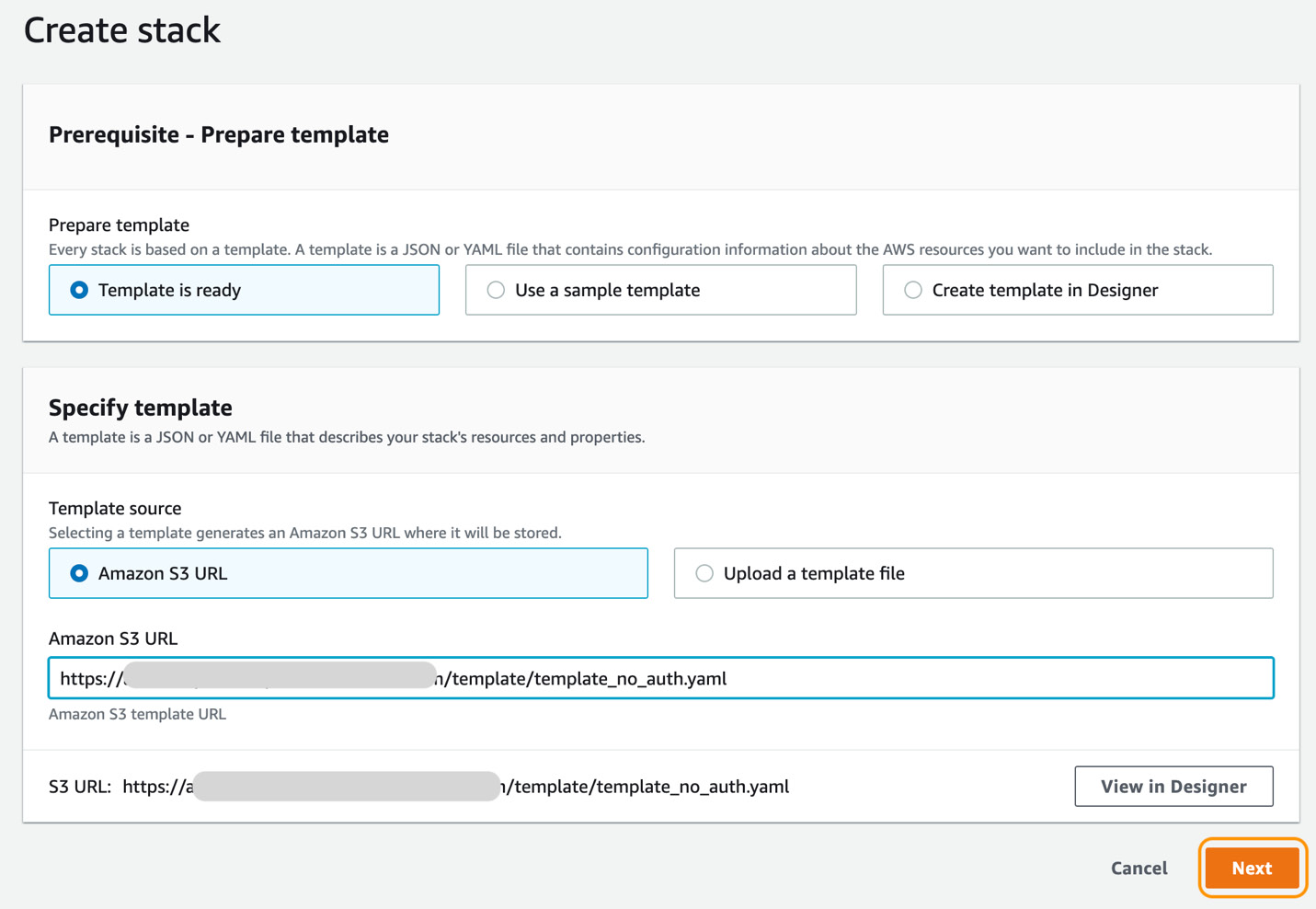
Figure 5.2 – Create stack

7. Enter the stack name of your choice and click on the Next button.
8. On the Configure stack options page, keep the default settings and click on the Next button at the bottom of the page.
9. On the Review page, scroll to the bottom of the screen, click on the I acknowledge that AWS CloudFormation might create IAM resources with custom names checkbox, and click on the Create stack button, as shown in Figure 5.3:

Figure 5.3 – Review stack

Note

The CloudFormation template will take 5-10 minutes to launch.

10. Once it is launched, go to Amazon SageMaker, click on SageMaker Studio, and you will see SageMaker Domain and studio-user configured for you, as shown in Figure 5.4:

Figure 5.4 – SageMaker Domain

11. Click on the Launch app dropdown next to studio-user and select Studio, as shown in the preceding screenshot. After this, you will be presented with a new JupyterLab interface (https://jupyterlab.readthedocs.io/en/latest/user/interface.html).

Note

It is recommended that you familiarize yourself with the Studio UI by reviewing the Amazon SageMaker Studio UI documentation (https://docs.aws.amazon.com/sagemaker/latest/dg/studio-ui.html), as we will be referencing many of the SageMaker-specific widgets and views throughout the chapter.

12. To make it easier to run the various examples within the book using the Studio UI, we will clone the source code from the companion GitHub repository. Within the Studio UI, click on the Git icon in the left sidebar and once the resource panel opens, click on the Clone a repository button to launch the Clone a repo dialog box, as shown in Figure 5.5:

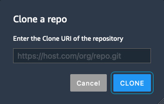
Figure 5.5 – Clone a repo

13. Enter the URL for the companion repository (https://github.com/PacktPublishing/Applied-Machine-Learning-and-High-Performance-Computing-on-AWS.git) and click the CLONE button.
14. The cloned repository will now appear in the File Browser panel of the Studio UI. Double-click on the newly cloned Applied-Machine-Learning-and-High-Performance-Computing-on-AWS folder to expand it.
15. Then double-click on the Chapter05 folder to open it for browsing.

We are now ready to analyze large amounts of structured data using SageMaker Studio. However, before we can start the analysis, we need to acquire the data. Let’s take a look at how to do that.

Analyzing large amounts of structured data

Since the objective of this section is to provide a hands-on example for analyzing large-scale structured data, our first task will be to synthesize a large amount of data. Using the Studio UI, execute the following steps:

1. Using the left File Browser panel, double-click on the 1_data_generator.ipynb file to launch the Jupyter notebook.
2. When prompted with the Set up notebook environment dialog box, ensure that Data Science is selected from the Image drop-down box, as well as Python 3 for the Kernel option. Figure 5.6 shows an example of the dialog box:

Figure 5.6 – Set up notebook environment

3. Once these options have been set, click the Select button to continue.
4. Next, you should see a Starting notebook kernel… message. The notebook kernel will take a couple of minutes to load.
5. Once the notebook has loaded, run the notebook by clicking on the Kernel menu and selecting the Restart kernel and Run All Cells… option.

After the notebook has executed all the code cells, we can dive into exactly what the notebook does, starting with a review of the dataset.

Reviewing the dataset

The dataset we will be using within this example is the California housing dataset (https://www.dcc.fc.up.pt/~ltorgo/Regression/cal_housing.html). This dataset was derived from the 1990 US census, using one row per census block group. A block group is the smallest geographical unit for which the US Census Bureau publishes sample data. A block group typically has a population of 600 to 3,000 people.

The dataset is incorporated into the scikit-learn or sklearn Python library (https://scikit-learn.org/stable/index.html). The scikit-learn library includes a dataset module that allows us to download popular reference datasets, such as the California housing dataset, from StatLib Datasets Archive (http://lib.stat.cmu.edu/datasets/).

Dataset citation

Pace, R. Kelley, and Ronald Barry, Sparse Spatial Autoregressions, Statistics and Probability Letters, 33 (1997) 291-297.

One key thing to be aware of is that this dataset only has 20,640 samples and is only around 400 KB in size. So, I’m sure you’ll agree that it doesn’t exactly qualify as a large amount of structured data. So, the primary objective of the notebook we’ve just executed is to use this dataset as a basis for synthesizing a much larger amount of structured data and then storing this new dataset on S3 for analysis.

Let’s walk through the code to see how this is done.

Installing the Python libraries

The first five code cells within the notebook are used to install and upgrade the necessary Python libraries to ensure we have the correct versions for the SageMaker SDK, scikit-learn, and the Synthetic Data Vault. The following code snippet shows the consolidation of these five code cells:

...
import sys
!{sys.executable} -m pip install "sagemaker>=2.51.0"
!{sys.executable} -m pip install --upgrade -q "scikit-learn"
!{sys.executable} -m pip install "sdv"
import sklearn
sklearn.__version__
import sdv
sdv.__version__
...

Note

There is no specific reason we upgrade and install the SageMaker and scikit-learn libraries except to ensure conformity across the examples within this chapter.

Once the required libraries have been installed, we load them and configure our global variables. The following code snippet shows how we import the libraries and configure the SageMaker default S3 bucket parameters:

...
import os
from sklearn.datasets import fetch_california_housing
import time
import boto3
import numpy as np
import pandas as pd
from sklearn.model_selection import train_test_split
import sagemaker
from sagemaker import get_execution_role
prefix = 'california_housing'
role = get_execution_role()
bucket = sagemaker.Session(boto3.Session()).default_bucket()
...

However, before we can synthesize a larger dataset and upload this to S3, we need to download the California housing dataset. As you can see from the following code snippet, we create two local folders called data and raw, then download the data using the fetch_california_housing() method from sklearn.datasets. The resultant data variable allows us to describe the data, as well as capture the data itself as a two-dimensional data structure called df_data:

...
data_dir = os.path.join(os.getcwd(), "data")
os.makedirs(data_dir, exist_ok=True)
raw_dir = os.path.join(os.getcwd(), "data/raw")
os.makedirs(raw_dir, exist_ok=True)
data = fetch_california_housing(data_home=raw_dir, download_if_missing=True, return_X_y=False, as_frame=True)
...
df_data = data.data
...

The df_data variable is the essential representation of our structured data, with columns showing the data labels and rows showing the observations or records for each label. Think of this structure as similar to a spreadsheet or relational table.

Using the df_data variable, we further describe this structure as well as perform some of the descriptive statistics and visualization described in the Exploring data analysis methods section of this chapter. For example, the following code snippet shows how to describe the type of data we are dealing with. You will recall that understanding the data type is crucial for appreciating the overall schema or structure of the data:

...
df_data.astype({'Population': 'int32'}).dtypes
...

Furthermore, we can define a Python function called plot_boxplot() to visualize the data included in the df_data variable. You will recall that visualizing the data provides further insight into the data. For example, as you can see from the next code snippet, we can visualize the overall distribution of the average number of rooms or avgNumrooms in the house:

...
import matplotlib.pyplot as plt
def plot_boxplot(data, title):
    plt.figure(figsize =(5, 4))
    plt.boxplot(data)
    plt.title(title)
    plt.show()
...
df_data.drop(df_data[df_data['avgNumRooms'] > 9].index, inplace = True)
df_data.drop(df_data[df_data['avgNumRooms'] <= 1].index, inplace = True)
plot_boxplot(df_data.avgNumRooms, 'rooms')
...

As we can see from Figure 5.7, the resultant boxplot from the code indicates that the average number of rooms for the California housing data is 5:

Figure 5.7 – Average number of rooms

Additionally, you will note from Figure 5.7 that there is somewhat of an equal distribution to the upper and lower bounds of the data. This indicates that we have a good distribution of data for the average number of bedrooms and therefore, we don’t need to augment this data point.

Finally, you will recall from the Counting the data points section that we can circumvent any unnecessary issues during the model training process by determining whether or not there are any missing values in the data. For example, the next code snippet shows how we can review a sum of any missing values in the df_data variable:

...
df_data.isna().sum()
...

While we’ve only covered a few analytics methodologies to showcase the analytics life cycle, a key takeaway from these examples is that the data is easy to analyze since it’s small enough to fit into memory. So, as data scientists, we did not have to capture a sample of the global population to analyze the data and then infer that analysis back onto the larger dataset. Let’s see whether this holds true once we synthesize a larger dataset.

Synthesizing large data

The last part of the notebook involves using the Synthetic Data Vault (https://sdv.dev/SDV/index.html), or the sdv Python library. This ecosystem of Python libraries uses ML models that specifically focus on learning from structured tabular and time series datasets and on creating synthetic data that carries the same format, statistical properties, and structure as the original dataset.

In our example notebook, we use a TVAE (https://arxiv.org/abs/1907.00503) model to generate a larger version of the California housing data. For example, the following code snippet shows how we define and train a TVAE model on the df_data variable:

...
from sdv.tabular import TVAE
model = TVAE(rounding=2)
model.fit(df_data)
model_dir = os.path.join(os.getcwd(), "model")
os.makedirs(model_dir, exist_ok=True)
model.save(f'{model_dir}/tvae_model.pkl')
...

Once we’ve trained the model, we can load it to generate 1 million new observations or rows in a variable called synthetic_data. The following code snippet shows an example of this:

...
from sdv.tabular import TVAE
model = TVAE.load(f'{model_dir}/tvae_model.pkl')
synthetic_data = model.sample(1000000)
...

Finally, as shown, we use the following code snippet to compress the data and leverage the SageMaker SDK’s upload_data() method to store the data in S3:

...
sess = boto3.Session()
sagemaker_session = sagemaker.Session(boto_session=sess)
synthetic_data.to_parquet('data/raw/data.parquet.gzip', compression='gzip')
rawdata_s3_prefix = "{}/data/raw".format(prefix)
raw_s3 = sagemaker_session.upload_data(path="./data/raw/data.parquet.gzip", key_prefix=rawdata_s3_prefix)
...

With a dataset of 1 million rows stored in S3, we finally have an example of a large amount of structured data. Now we can use this data to demonstrate how to leverage the highlighted analysis methods at scale on structured data using Amazon EMR.

Analyzing large-scale data using an EMR cluster with SageMaker Studio

To get started with analyzing the large-scale synthesized dataset we’ve just created, we can execute the following steps in the Studio UI:

1. Using the left-hand navigation panel, double-click on the 2_data_exploration_spark.ipynb notebook to launch it.
2. As we saw with the previous example, when prompted with the Set up notebook environment dialog box, select SparkMagic as Image and PySpark as Kernel.
3. Once the notebook is ready, click on the Kernel menu option and once again select the Restart kernel and Run All Cells… option to execute the entire notebook.

While the notebook is running, we can start reviewing what we are trying to accomplish within the various code cells. As you can see from the first code cell, we connect to the EMR cluster we provisioned in the Setting up EMR and SageMaker Studio section:

%load_ext sagemaker_studio_analytics_extension.magics
%sm_analytics emr connect --cluster-id <EMR Cluster ID> --auth-type None

In the next code cell, shown by the following code, we read the synthesized dataset from S3. Here we create a housing_data variable by using PySpark’s sqlContext method to read the raw data from S3:

housing_data=sqlContext.read.parquet('s3://<SageMaker Default Bucket>/california_housing/data/raw/data.parquet.gzip')

Once we have this variable assigned, we can use PySpark and the EMR cluster to execute the various data analysis tasks on the entire population of the data without having to ingest a sample dataset on which to perform the analysis.

While the notebook provides multiple examples of different analysis methodologies that are specific to the data, we will focus on the few examples that relate to the exploration we’ve already performed on the original California housing dataset to illustrate how these same methodologies can be applied at scale.

Reviewing the data structure and counts

As already mentioned, understanding the type of data, its structure, and the counts is an important part of the analysis. To perform this analysis on the entirety of housing_data, we can execute the following code:

print((housing_data.count(), len(housing_data.columns)))
housing_data.printSchema()

Executing this code produces the following output, where we can see that we have 1 million observations, as well as the data types for each feature:

(1000000, 9)
Root
|-- medianIncome: double (nullable = true)
|-- medianHousingAge: double (nullable = true)
|-- avgNumRooms: double (nullable = true)
|-- avgNumBedrooms: double (nullable = true)
|-- population: double (nullable = true)
|-- avgHouseholdMembers: double (nullable = true)
|-- latitude: double (nullable = true)
|-- longitude: double (nullable = true)
|-- medianHouseValue: double (nullable = true)

Next, we can determine whether or not there are any missing values and how to deal with them.

Handling missing values

You will recall that ensuring that there are no missing values is an important methodology for any data analysis. To expose any missing data, we can run the following code to create a count of any missing values for each column or feature within this large dataset:

from pyspark.sql.functions import isnan, when, count, col
housing_data.select([count(when(isnan(c), c)).alias(c) for c in housing_data.columns]).show()

If we do find any missing values, there are a number of techniques we can use to deal with them. For example, we delete rows containing missing values, using the dropna() method on the housing_data variable. Alternatively, depending on the number of missing values, we can use imputation techniques to infer a value based on the mean or median of the feature.

Analyzing the centrality and variability of the data

Remember that understanding how the data is distributed will give us a good idea of whether the data is proportional or not. This analysis task also provides an idea of whether we have outliers within our data that skew the distribution or spread. Previously, it was emphasized that visualizing the data distribution using bar charts and boxplots can further assist in determining the variability of the data.

To accommodate this task, the following code highlights an example of capturing the features we wish to analyze and plotting their distribution as a bar chart:

import matplotlib.pyplot as plt
df = housing_data.select('avgNumRooms', 'avgNumBedrooms', 'population').toPandas()
df.hist(figsize=(10, 8), bins=20, edgecolor="black")
plt.subplots_adjust(hspace=0.3, wspace=0.5)
plt.show()
%matplot plt

After executing this code on the large data, we can see an example of the resultant distribution for the average number of rooms (avgNumRooms), the average number of bedrooms (avgNumBedrooms), and block population (population) features in Figure 5.8:

Figure 5.8 – Feature distribution

As you can see from Figure 5.8, both the avgNumBedrooms and population features are not centered around the mean or average for the feature. Additionally, the spread for the avgNumBedrooms feature is significantly skewed toward the lower end of the spectrum. This factor could indicate that there are potential outliers or too many data points that are consolidated between 1.00 and 1.05. This fact is further confirmed if we use the following code to create a boxplot of the avgNumBedrooms feature:

plot_boxplot(df.avgNumBedrooms, 'Boxplot for Average Number of Bedrooms')
%matplot plt

The resultant boxplot from running this code cell is shown in Figure 5.9:

Figure 5.9 – Boxplot for the average number of bedrooms

Figure 5.9 clearly shows that there are a number of outliers that cause the data to be skewed. Therefore, we need to resolve these discrepancies as part of our data analysis and before ML models can be trained on our large dataset. The following code snippet shows how to query the data from the boxplot values and then simply remove it, to create a variable called housing_df_with_no_outliers:

import pyspark.sql.functions as f
columns = ['avgNumRooms', 'avgNumBedrooms', 'population']
housing_df_with_no_outliers = housing_data.where(
    (housing_data.avgNumRooms<= 8) &
    (housing_data.avgNumRooms>=2) &
    (housing_data.avgNumBedrooms<=1.12) &
    (housing_data.population<=1500) &
    (housing_data.population>=250))

Once we have our housing_df_with_no_outliers, we can use the following code to create a new boxplot of the variability of the avgNumBedrooms feature:

df = housing_df_with_no_outliers.select('avgNumRooms', 'avgNumBedrooms', 'population').toPandas()
plot_boxplot(df.avgNumBedrooms, 'Boxplot for Average Number of Bedrooms')
%matplot plt

Figure 5.10 shows an example of a boxplot produced from executing this code:

Figure 5.10 – Boxplot of the average number of bedrooms

From Figure 5.10, we can clearly see that the outliers have been removed. Subsequently, we can perform a similar procedure on the avgNumRooms and population features.

While these examples only show some of the important methodologies highlighted within the data analysis life cycle, an important takeaway from this exercise is that due to the integration of SageMaker Studio and EMR, we’re able to accomplish the data analysis tasks on large-scale structured data without having to capture a sample of the global population and then infer that analysis back onto the larger dataset. However, along with analyzing the data at scale, we also need to ensure that any preprocessing tasks are also executed at scale.

Next, we will review how to automate these preprocessing tasks at scale using SageMaker.

Preprocessing the data at scale

The SageMaker service takes care of the heavy lifting and scaling of data transformation or preprocessing tasks using one of its core components called Processing jobs (https://docs.aws.amazon.com/sagemaker/latest/dg/processing-job.html). While Processing jobs allows a user to leverage built-in images for scikit-learn or even custom images, they also reduce the heavy-lifting task of provisioning ephemeral Spark clusters (https://docs.aws.amazon.com/sagemaker/latest/dg/use-spark-processing-container.html). This means that data scientists can perform large-scale data transformations automatically without having to create or have the infrastructure team create an EMR cluster. All that’s required of the data scientist is to convert the processing code cell into a Python script called preprocess.py.

The following code snippet shows how the code to remove outliers can be converted into a Python script:

%%writefile preprocess.py
...
def main():
    parser = argparse.ArgumentParser(description="app inputs and outputs")
    parser.add_argument("--bucket", type=str, help="s3 input bucket")
    parser.add_argument("--s3_input_prefix", type=str, help="s3 input key prefix")
    parser.add_argument("--s3_output_prefix", type=str, help="s3 output key prefix")
    args = parser.parse_args()
    spark = SparkSession.builder.appName("PySparkApp").getOrCreate()
    housing_data=spark.read.parquet(f's3://{args.bucket}/{args.s3_input_prefix}/data.parquet.gzip')
    housing_df_with_no_outliers = housing_data.where((housing_data.avgNumRooms<= 8) &
                   (housing_data.avgNumRooms>=2) &
                   (housing_data.avgNumBedrooms<=1.12) &
                    (housing_data.population<=1500) &
                    (housing_data.population>=250))
    (train_df, validation_df) = housing_df_with_no_outliers.randomSplit([0.8, 0.2])
    train_df.write.parquet("s3://" + os.path.join(args.bucket, args.s3_output_prefix, "train/"))
    validation_df.write.parquet("s3://" + os.path.join(args.bucket, args.s3_output_prefix, "validation/"))
if __name__ == "__main__":
    main()
...

Once the Python script is created, we can load the appropriate SageMaker SDK libraries and configure the S3 locations for the input data as well as the transformed output data, as follows:

%local
import sagemaker
from time import gmtime, strftime
sagemaker_session = sagemaker.Session()
role = sagemaker.get_execution_role()
bucket = sagemaker_session.default_bucket()
timestamp = strftime("%Y-%m-%d-%H-%M-%S", gmtime())
prefix = "california_housing/data_" + timestamp
s3_input_prefix = "california_housing/data/raw"
s3_output_prefix = prefix + "/data/spark/processed"

Finally, we can instantiate an instance of the SageMaker PySparkProcessor() class (https://sagemaker.readthedocs.io/en/stable/api/training/processing.html#sagemaker.spark.processing.PySparkProcessor) as a spark_processor variable, as can be seen in the following code:

%local
from sagemaker.spark.processing import PySparkProcessor
spark_processor = PySparkProcessor(
    base_job_name="sm-spark",
    framework_version="2.4",
    role=role,
    instance_count=2,
    instance_type="ml.m5.xlarge",
    max_runtime_in_seconds=1200,
)

With the spark_processor variable defined, we can then call the run() method to execute a SageMaker Processing job. The following code demonstrates how to call the run() method and supply the preprocess.py script along with the input and output locations for the data as arguments:

spark_processor.run(
    submit_app="preprocess.py",
    arguments=[
        "--bucket",
        bucket,
        "--s3_input_prefix",
        s3_input_prefix,
        "--s3_output_prefix",
        s3_output_prefix,
    ],
)

In the background, SageMaker will create an ephemeral Spark cluster and execute the preprocess.py script on the input data. Once the data transformations are completed, SageMaker will store the resultant dataset on S3 and then decommission the Spark cluster, all while redirecting the execution log output back to the Jupyter notebook.

While this technique makes the complicated task of analyzing large amounts of structured data much easier to scale, there is still the question of how to perform a similar procedure on unstructured data.

Let’s review how to solve this problem next.

Analyzing large amounts of unstructured data

In this section, we will use unstructured data (horse and human images) downloaded from https://laurencemoroney.com/datasets.html. This dataset can be used to train a binary image classification model to classify horses and humans in the image. From the SageMaker Studio, launch the 3_unstructured_data_s3.ipynb notebook with PyTorch 1.8 Python 3.6 CPU Optimized selected from the Image drop-down box as well as Python 3 for the Kernel option. Once the notebook is opened, restart the kernel and run all the cells as mentioned in the Analyzing large-scale data using an EMR cluster with SageMaker Studio section.

After the notebook has executed all the code cells, we can dive into exactly what the notebook does.

As you can see in the notebook, we first download the horse-or-human data from https://storage.googleapis.com/laurencemoroney-blog.appspot.com/horse-or-human.zip and then unzip the file.

Once we have the data, we will convert the images to high resolution using the EDSR model provided by the Hugging Face super-image library:

1. We will first download the pretrained model with scale = 4, which means that we intend to increase the resolution of the images four times, as shown in the following code block:

   from super_image import EdsrModel, ImageLoader

   from PIL import Image

   import requests

   model = EdsrModel.from_pretrained('eugenesiow/edsr-base', scale=4)
2. Next, we will iterate through the folder containing the images, use the pretrained model to convert each image to high resolution, and save it, as shown in the following code block:

   import os

   from os import listdir

   folder_dir = "horse-or-human/"

   for folder in os.listdir(folder_dir):

       folder_path = f'{folder_dir}{folder}'

       for image_file in os.listdir(folder_path):

           path = f'{folder_path}/{image_file}'

           image = Image.open(path)

           inputs = ImageLoader.load_image(image)

           preds = model(inputs)

           ImageLoader.save_image(preds, path)

You can check the file size of one of the images to confirm that the images have been converted to high resolution. Once the images have been converted to high resolution, you can optionally duplicate the images to increase the number of files and finally upload them to S3 bucket. We will use the images uploaded to the S3 bucket for running a SageMaker training job.

Note

In this example, we will walk you through the option of running a training job with PyTorch using the SageMaker training feature using the data stored in an S3 bucket. You can also choose to use other frameworks as well, such as TensorFlow and MXNet, which are also supported by SageMaker.

In order to use PyTorch, we will first import the sagemaker.pytorch module, using which we will define the SageMaker PyTorch Estimator, as shown in the following code block:

from sagemaker.pytorch import PyTorch
estimator = PyTorch(entry_point='train.py',
                    source_dir='src',
                    role=role,
                    instance_count=1,
                    instance_type='ml.g4dn.8xlarge',
                    framework_version='1.8.0',
                    py_version='py3',
                    sagemaker_session=sagemaker_session,
                    hyperparameters={'epochs':5,
                                     'subset':2100,
                                     'num_workers':4,
                                     'batch_size':500},
                   )

In the estimator object, as you can see from the code snippet, we need to provide configuration parameters. In this case, we need to define the following parameters:

• instance_count: This is the number of instances
• instance_type: This is the type of instance on which the training job will be launched
• framework_version: This is the framework version of PyTorch to be used for training
• py_version: This is the Python version
• source_dir: This is the folder path within the notebook, which contains the training script
• entry_point: This is the name of the Python training script
• hyperparameters: This is the list of hyperparameters that will be used by the training script

Once we have defined the PyTorch estimator, we will define the TrainingInput object, which will take the S3 location of the input data, content type, and input mode as parameters, as shown in the following code:

from sagemaker.inputs import TrainingInput
train = TrainingInput(s3_input_data,content_type='image/png',input_mode='File')

The input_mode parameter can take the following values; in our case, we are using the File value:

• None: Amazon SageMaker will use the input mode specified in the base Estimator class
• File: Amazon SageMaker copies the training dataset from the S3 location to a local directory
• Pipe: Amazon SageMaker streams data directly from S3 to the container via a Unix-named pipe
• FastFile: Amazon SageMaker streams data from S3 on demand instead of downloading the entire dataset before training begins

Note

You can see the complete list of parameters for the PyTorch estimator at this link: https://sagemaker.readthedocs.io/en/stable/frameworks/pytorch/sagemaker.pytorch.html.

Once we have configured the PyTorch Estimator and TrainingInput objects, we are now ready to start the training job, as shown in the following code:

estimator.fit({'train':train})

When we run estimator.fit, it will launch one training instance of the ml.g4dn.8xlarge type, install the PyTorch 1.8 container, copy the training data from S3 location and the train.py script to the local directory on the training instance, and will finally run the training script that you have provided in the estimator configuration. Once the training job is completed, SageMaker will automatically terminate all the resources that it has launched, and you will only be charged for the amount of time the training job was running.

In this example, we used a simple training script that involved loading the data using the PyTorch DataLoader object and iterating through the images. In the following section, we’ll see how to process data at scale using AWS.

Processing data at scale on AWS

In the previous section, Analyzing large amounts of unstructured data, the data was stored in an S3 bucket, which was used for training. There will be scenarios where you will need to load data faster for training instead of waiting for the training job to copy the data from S3 locally into your training instance. In these scenarios, you can store the data on a file system, such as Amazon Elastic File System (EFS) or Amazon FSx, and mount it to the training instance, which will be faster than storing the data in S3 location. The code for this is in the 3_unstructured_data.ipynb notebook. Refer to the Optimize it with data on EFS and Optimize it with data on FSX sections in the notebook.

Note

Before you run the Optimize it with data on EFS and Optimize it with data on FSX sections, please launch the CloudFormation template_filesystems.yaml template, in a similar fashion as we did in the Setting up EMR and SageMaker Studio section.

Cleaning up

Let’s terminate the EMR cluster, which we launched in the Setting up EMR and SageMaker Studio section, as it will not be used in the later chapters of the book.

Let’s start by logging into the AWS console and following the steps given here:

1. Search EMR in the AWS console.
2. You will see the active EMR-Cluster-sm-emr cluster. Select the checkbox against the EMR cluster name and click on the Terminate button, as shown in Figure 5.11:

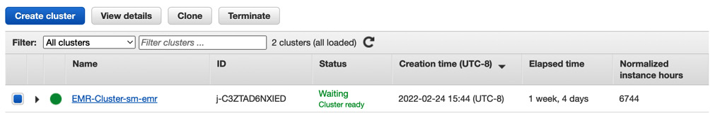
Figure 5.11 – List EMR cluster

3. Click on the red Terminate button in the pop-up window, as shown in Figure 5.12:

Figure 5.12 – Terminate EMR cluster

4. It will take a few minutes to terminate the EMR cluster, and once completed, Status will change to Terminated.

Let’s summarize what we’ve learned in this chapter.

Summary

In this chapter, we explored various data analysis methods, reviewed some of the AWS services for analyzing data, and launched a CloudFormation template to create an EMR cluster, SageMaker Studio domain, and other useful resources. We then did a deep dive into code for analyzing both structured and unstructured data and suggested a few methods for optimizing its performance. This will help you to prepare your data for training ML models.

In the next chapter, we will see how we can train large models on large amounts of data in a distributed fashion to speed up the training process.