6

Distributed Training of Machine Learning Models

When it comes to Machine Learning (ML) model training, the primary goal for a data scientist or ML practitioner is to train the optimal model based on the relevant data to address the business use case. While this goal is of primary importance, the panacea is to perform this task as quickly and effectively as possible. So, how do we speed up model training? Moreover, sometimes, the data or the model might be too big to fit into a single GPU memory. So how do we prevent out-of-memory (OOM) errors?

The simplest answer to this question is to basically throw more compute resources, in other words, more CPUs and GPUs, at the problem. This is essentially using larger compute hardware and is commonly referred to as a scale-up strategy. However, there is only a finite number of CPUs and GPUs that can be squeezed into a server. So, sometimes a scale-out strategy is required, whereby we add more servers into the mix, essentially distributing the workload across multiple physical compute resources.

Nonetheless, spreading the model training workload across more CPUs or GPUs, and even across more compute servers, will definitely speed up the overall training process. Making use of either a scale-up, scale-out, or a combination of the two strategies also adds further complexity to the overall orchestration and configuration of the model training activity. Therefore, this chapter will help navigate these challenges to help overcome the additional complexities imposed by the distributed training process by covering the following topics:

• Building ML systems using AWS
• Introducing the fundamentals of distributed training
• Executing a distributed training workload on AWS

Technical requirements

You should have the following prerequisites before getting started with this chapter:

• A web browser (for the best experience, it is recommended that you use a Chrome or Firefox browser)
• Access to the AWS account that you used in Chapter 5, Data Analysis
• An AWS account (if you are unfamiliar with how to get started with an AWS account, you can go to this link https://aws.amazon.com/getting-started/)
• Access to the SageMaker Studio development environment that we created in Chapter 5, Data Analysis
• Example Jupyter notebooks for this chapter are provided in the companion GitHub repository (https://github.com/PacktPublishing/Applied-Machine-Learning-and-High-Performance-Computing-on-AWS/tree/main/Chapter06)

Building ML systems using AWS

Before we can explore the fundamentals of how to implement the distributed training strategies highlighted at the outset, we first need to level set and understand just how the ML model training exercise can be performed on the AWS platform. Once we understand how AWS handles model training, we can further expand on this concept to address the concept of distributed training.

To assist ML practitioners in building ML systems, AWS provides the SageMaker (https://aws.amazon.com/sagemaker/) service. While SageMaker is a single AWS service, it comprises multiple modules that map specifically to an ML task. For example, SageMaker provides the Training job component that is purpose-built to take care of the heavy lifting and scaling of the model training task. ML practitioners can use SageMaker Training jobs to essentially provision ephemeral compute environments or clusters to handle the model training task. Essentially, all the ML practitioner needs to do is specify a few configuration parameters, and SageMaker Training jobs takes care of the rest. For example, we need to supply the following four basic parameters:

• The URL for the S3 bucket, which contains the model training, testing, and optionally, the validation data
• The type and quantity of ML compute instances required to perform the model training task
• The location of the S3 bucket to store the trained model
• The location, either locally or on S3, where the model training code is stored

The following code snippet shows just how easy it can be to formalize these four basic requirements into a SageMaker Training job request:

...
from sagemaker.pytorch import PyTorch
estimator = PyTorch(entry_point='train.py',
                    source_dir='src',
                    role=role,
                    instance_count=1,
                    instance_type='ml.p3.2xlarge',
                    framework_version='1.8.0',
                    py_version='py3',
                    sagemaker_session=sagemaker_session,
                    hyperparameters={'epochs':10,
                                     'batch_size':32,
                                     'lr':3e-5,
                                     'gamma': 0.7},
                   )
...

Using this code snippet, we basically tell SageMaker that we want to use the built-in PyTorch estimator by declaring the estimator variable to use the PyTorch framework. We then supply the necessary requirements, such as the following:

• entry_point: This is the location of the training script.
• instance_count: This is the number of compute servers to be provisioned in the cluster.
• instance_type: This is the type of compute resources required in the cluster. In this example, we are specifying the ml.p3.16xlarge instances.

Note

For more information on the SageMaker PyTorch estimator, as well as how to leverage the SageMaker SDK to instantiate the estimator, see the AWS documentation on how to use PyTorch on SageMaker (https://docs.aws.amazon.com/sagemaker/latest/dg/pytorch.html) and the SageMaker SDK documentation (https://sagemaker.readthedocs.io/en/stable/frameworks/pytorch/sagemaker.pytorch.html#pytorch-estimator).

Once we have declared the estimator, we specify the location of the training and validation datasets on S3, as shown in the following code snippet:

...
from sagemaker.inputs import TrainingInput
train = TrainingInput(s3_train_data,
                      content_type='image/png',
                      input_mode='File')
val = TrainingInput(s3_val_data,
                    content_type='image/png',
                    input_mode='File')
...

We then call the fit() method of the PyTorch estimator to tell SageMaker to execute the Training job on the datasets, as shown in the following code snippet:

...
estimator.fit({'train':train, 'val': val})
...

Behind the scenes, SageMaker creates an ephemeral compute cluster, executes the training task on these resources, and then produces the resultant optimized model, which is then stored on Amazon S3. After this task has been performed, SageMaker tears down the ephemeral cluster with users only paying for the resources consumed during the training time.

Note

For more detailed information as to how SageMaker Training jobs work behind the scenes, see the AWS documentation (https://docs.aws.amazon.com/sagemaker/latest/dg/how-it-works-training.html).

So now that we have a basic idea of how a model training exercise can be performed using Amazon SageMaker, how can we improve on model training time and essentially speed up the process by leveraging more compute resources?

To answer this question, we can very easily implement a scale-up strategy with the SageMaker Training job. All we have to do is change the instance_type parameter for the estimator variable from ml.p3.2xlarge to ml.p3.16xlarge. By doing this, we are increasing the size of, or scaling up the compute resource from, an instance with 8 vCPUs, 61 GB of RAM, and a single GPU to an instance with 64 vCPUs, 488 GB of RAM, and 8 GPUs.

The resultant code now looks as follows:

...
from sagemaker.pytorch import PyTorch
estimator = PyTorch(entry_point='train.py',
                    source_dir='src',
                    role=role,
                    instance_count=1,
                    instance_type='ml.p3.16xlarge',
                    framework_version='1.8.0',
                    py_version='py3',
                    sagemaker_session=sagemaker_session,
                    hyperparameters={'epochs':10,
                                     'batch_size':32,
                                     'lr':3e-5,
                                     'gamma': 0.7},
                   )
...

So, as you can see, implementing a scale-up strategy is very straightforward when using SageMaker. However, what if we need to go beyond the maximum capacity of an accelerated computing instance?

Well, then, we would need to implement a scale-out strategy and distribute the training process across multiple compute nodes. In the next section, we will explore how to apply a scale-out strategy using distributed training for SageMaker Training jobs.

Introducing the fundamentals of distributed training

In the previous section, we highlighted how to apply a scale-up strategy to SageMaker Training jobs by simply specifying a large compute resource or large instance type. Implementing a scale-out strategy for the training process is just as straightforward. For example, we can increase the instance_count parameter for the Training job from 1 to 2 and thereby instruct SageMaker to instantiate an ephemeral cluster consisting of 2 compute resources as opposed to 1 node. Thus, the following code snippet highlights what the estimator variable configuration will look like:

...
from sagemaker.pytorch import PyTorch
estimator = PyTorch(entry_point='train.py',
                    source_dir='src',
                    role=role,
                    instance_count=2,
                    instance_type='ml.p3.2xlarge',
                    framework_version='1.8.0',
                    py_version='py3',
                    sagemaker_session=sagemaker_session,
                    hyperparameters={'epochs':10,
                                     'batch_size':32,
                                     'lr':3e-5,
                                     'gamma': 0.7},
                   )
...

Unfortunately, simply changing the number of compute instances doesn’t completely solve the problem. As already stated at the outset of this chapter, applying a scale-out strategy to distribute the SageMaker Training job adds further complexity to the overall orchestration and configuration of the model training activity. For example, when distributing the training activity, we need to also take into consideration the following aspects:

• How do the various compute resources get access to and share the data?
• How do the compute resources communicate and coordinate their training tasks with each other?

So, while simply specifying the number of compute resources for the Training job will create an appropriately sized training cluster, we also need to inform SageMaker about our model placement strategy. A model placement strategy directs SageMaker on exactly how the model is allocated or assigned to each of the compute resources within each node of the cluster. In turn, SageMaker uses the placement strategy to coordinate how each node interacts with the associated training data and, subsequently, how each node coordinates and communicates its portion of the model training task.

So how do we determine an effective model placement strategy for SageMaker?

The best way to answer this question is to understand what placement strategies are available and dissect how each of these strategies works. There are numerous placement strategies that are specific to each of the different training frameworks, as well as many open source frameworks. Nonetheless, all these different mechanisms can be grouped into two specific categories of placement strategies, namely data parallel and model parallel.

Let’s explore SageMaker’s data parallel strategy first.

Reviewing the SageMaker distributed data parallel strategy

As the name implies, a data parallel strategy focuses on the placement of model’s training data. So, in order to fully understand just how this placement strategy is applied to the data, we should start by understanding just how a training activity interacts with the training data to optimize an ML model.

When we train an ML model, we basically create a training loop that applies the specific ML algorithm to the data. Typically, as is the case with deep learning algorithms, we break the data into smaller groups of records or batches of data. These batches are referred to as mini batches. We then pass each of these mini batches forward through the neural network layers, and then backward to optimize or train the model parameters. After completing one mini batch, we then apply the same procedure to the next mini batch, and so on, until we’ve run through the entirety of the data. A full execution of this process on the entire dataset is referred to as an epoch. Depending on the type of algorithm and, of course, the use case, we may have to run the algorithm to train the model for multiple epochs. It’s this task that invariably takes the most time, and it’s this task that we essentially want to improve on to reduce the overall time it takes to train the model.

So, when using a data parallel placement strategy, we are basically converting the training task from a sequential process to a parallel process. Instead of running the algorithm through a mini batch, then the next mini batch, then the next mini batch sequentially, we are now giving each individual mini batch to a separate compute resource, with each compute resource, in turn, running the model training process on its individual mini batch. Therefore, with each compute resource running its own mini batch at the same time, we are effectively distributing the epoch across multiple compute resources in parallel, therefore, improving the overall model training time. Consequently, using the data parallel technique does, however, introduce an additional complication, namely parallel optimization of all the weighted parameters for the model.

To further elaborate on this problem, we’ll use the example depicted in Figure 6.1, detailing the individual node parameters for the model:

Figure 6.1 – Individual node parameters

As you can see from the example in Figure 6.1, we have four individual compute resources or nodes. Using the data parallel placement strategy, we have effectively placed a copy of the model algorithm onto each of these nodes and distributed the mini batch data across these resources. Now, each node computes the gradient reduction operation, in this case, the sum of weighted parameters of the model, on its individual mini batch of the data, in essence, producing four unique gradient calculation results. Since our goal is not to produce four separate representations of an optimized model but rather a single optimized model, how do we combine the results across all four nodes?

To solve this problem, SageMaker provides an additional optimization operation to the distributed training process and uses the AllReduce algorithm to share and communicate the results across the cluster. By including this additional step in the process, we can see the outcome in Figure 6.2:

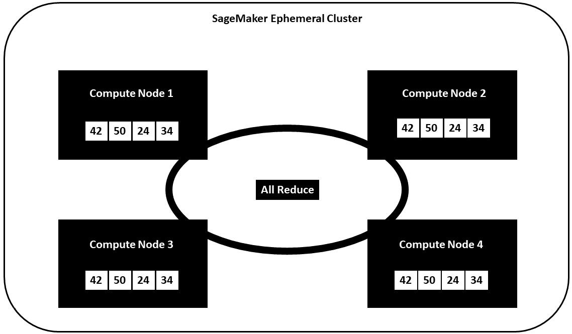
Figure 6.2 – Shared node parameters

From Figure 6.2, we can see that the AllReduce step takes the results from each node’s gradient reduction operation and shares the results with every other node, ensuring that each node’s representation of the model includes the optimizations from all the other nodes. This, therefore, guarantees that a single, consistent model is produced as the final output from the distributed training process.

Note

While the initial concept of using the AllReduce step for distributed deep learning was initially introduced in a blog post by Baidu Research, the original post has since been removed. So, for more background information on the intricacies of how it works, you can review the open source implementation called Horovod (https://eng.uber.com/horovod/).

Up until this point in the chapter, we have used the broad term compute resources to denote CPUs, GPUs, and physical compute instances. However, when implementing a successful data parallel placement strategy, it’s important to fully understand just how SageMaker uses these compute resources to execute the distributed training workload.

Succinctly, when we instruct SageMaker to implement a data parallel placement strategy for the Training job, we are instructing SageMaker to distribute or shard the mini batches across all of the compute resources. SageMaker, in turn, shards the training data into all the GPUs and, from time to time, the CPUs on all of the instance types specified in the estimator object. So, in order to make this concept easier to understand, Figure 6.3 illustrates an example of just how SageMaker handles the task:

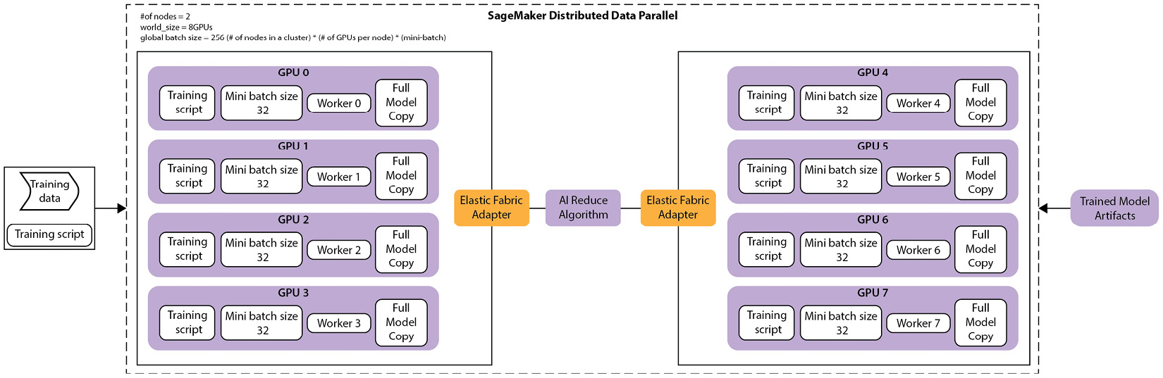
Figure 6.3 – Data parallel training task on SageMaker

As you can see from the example shown in Figure 6.3 when calling the fit() method for the SageMaker estimator object, specifying two GPU instances (each with eight GPUs), SageMaker creates a copy of the model training routine, or training script, on both of the instances in the ephemeral cluster. Accordingly, each training script is further copied onto each GPU on each of the instances. Once every GPU has a copy of the training script, each GPU, in turn, executes the training script on its individually sharded mini batch of the training data.

The GPU worker then trains the model copy to produce a set of optimal parameters, which then shares with the other GPU workers, both within the same instance, as well as the other GPUs in the second instance, using the AllReduce optimization algorithm. This process is repeated in parallel until all of the specified epochs are completed, after which the ephemeral SageMaker cluster is dismantled, and the fit() operation is reported as being successful. The result is a single optimized model, stored on S3, and a reduction of the overall model training time, by a factor of 16, which is the total number of GPUs allocated to the task.

So, as you can see, we have effectively reduced the overall training time by implementing a data parallel placement strategy. While this strategy is effective for large training datasets and is a good start at reducing the time it takes to train a model, this strategy, however, doesn’t always work when we have large models to train.

Note

Since the model parallel placement strategy is essentially distributing the model’s computational graph or model pipeline across multiple nodes, this placement strategy is often referred to as a pipeline parallel strategy.

To address the challenge of reducing the overall training time when we have large ML models with millions or even billions of trainable parameters, we can review how to implement a model parallel placement strategy.

Reviewing the SageMaker model data parallel strategy

The data parallel strategy was largely conceived as a method of reducing the overall model training time, where at the time of its induction, training on large quantities of data imposed the biggest challenge. However, with the invention of large-scale natural language processing (NLP) models, such as Generative Pre-trained Transformers (GPT) from OpenAI (https://openai.com/blog/gpt-3-apps/), training a large ML model will billions of parameters now imposes the biggest challenge. Basically, these models are far too large to fit into the GPU’s onboard memory.

Now that we have a rudimentary idea of just how SageMaker implements a data parallel placement strategy, it’s relatively easy to translate the concept to a model parallel placement strategy. The key difference is that while a data parallel strategy breaks the large quantity of training data into smaller shards, the model parallel placement strategy performs a similar trick to a large ML model, allowing these smaller pieces of the model to fit into GPU memory. This also means that we don’t have to degrade the model’s capabilities by having to prune or compress it.

Figure 6.4 highlights just how similar the model parallel execution is to a data parallel execution when SageMaker executes a Training job, using a model parallel placement strategy:

Figure 6.4 – Model parallel training task on SageMaker

You can see from Figure 6.4 that when calling the fit() method for the SageMaker estimator object, just like the data parallel example in Figure 6.3, SageMaker allocates a copy of the model training script to each GPU on each of the two instances. However, instead of distributing the same copy of the model to each GPU worker, as was the case with the data parallel placement strategy, SageMaker splits the model into smaller pieces, or model partitions, assigning each model partition to a GPU worker.

To coordinate how the training of each model partition, SageMaker implements a pipeline scheduler. In the same way that the AllReduce optimization algorithm coordinates parameter optimizations across different GPU workers, the pipeline scheduler ensures that as each batch of data is fed into the model and computation for each partition of the model is correctly coordinated and scheduled between all the GPU workers. This ensures that the matrix calculations for each layer, during both the forward and backward passes over these network partitions, happen in accordance with the overall structure of the model architecture. For example, the scheduler would ensure that the mathematical calculations for layer two are executed before layer three on the forward pass and that layer three’s gradient calculation occurs before layer two. Once all the desired epochs have been executed, essentially both the forward and backward passes through the model architecture over the entirety of the training data, SageMaker dismantles the ephemeral cluster and stores the optimized model on S3.

In summation, the data parallel placement strategy was originally conceived to reduce the overall training time of a model by sharing the data and parallelizing the execution across multiple compute resources. The primary motivation behind a model parallel placement strategy is to address large models that don’t fit into the compute resource’s memory. This then begs the question as to whether it’s possible to combine both the data parallel and model parallel placement strategies to reduce the overall training time for both large models, as well as large datasets in a distributed fashion.

Let’s review this hybrid methodology next.

Reviewing a hybrid data parallel and model parallel strategy

The fact that both the data parallel and model parallel placement strategies were created to address specific challenges, it is fundamentally impossible to combine both strategies into a unified, hybrid strategy. Essentially, both strategies only solve their specific issues by either sharding the data or sharding the model.

Fortunately, because the entirety of the Training job is orchestrated and managed by SageMaker, the ability to combine both strategies into a hybrid strategy is now possible. For example, if we review Figure 6.5, we can visualize just how SageMaker allows us to execute a Training job that implements both the data parallel and model parallel placement strategies independently:

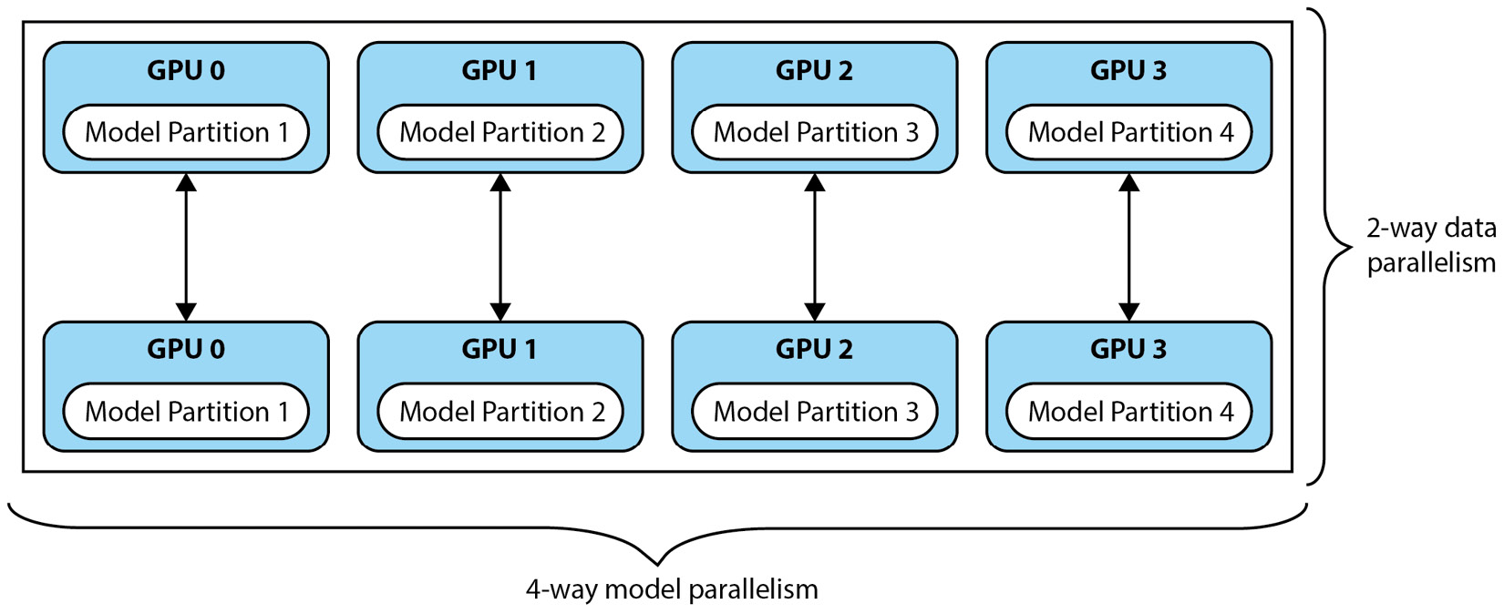
Figure 6.5 – Independent data parallel and model parallel strategies on SageMaker

Figure 6.5 illustrates taking the same number of compute instances, and essentially implementing a two-node data parallel placement strategy, along with a four-way model parallel placement strategy. This translates to creating two copies of the training script and assigning each copy to one of the two compute instances. We then execute the distributed training task using the data parallel placement strategy. While the training task is being executed, we further partition the specific copy of the model architecture across each of the GPUs in the individual compute instance, using the model parallel placement strategy.

So, while each of these placement strategies is unique in its approach, by using SageMaker, we can reap the benefits of both approaches to reduce the overall training time on large datasets, as well as large ML models. In the next section, we will review examples of how to practically implement each of the placement strategies on SageMaker, including an example of this hybrid approach.

Executing a distributed training workload on AWS

Now that we’ve been introduced to some of the fundamentals of distributed training and what happens behind the scenes when we leverage SageMaker to launch a distributed Training job, let’s explore how we can execute such a workload on AWS. Since we’ve reviewed two placement techniques, namely data parallel and model parallel, we will start by reviewing how to execute distributed data parallel training. After which, we will then review how to execute distributed model parallel training, but also include the hybrid methodology and include an independent data parallel placement strategy alongside the model parallel example.

Note

In this example, we leverage a Vision Transformer (ViT) model to address an image classification use case. Since the objective of this section is to showcase how to practically implement both the data parallel and model parallel placement strategies, we will not be diving into the particulars of the model itself but rather using it within the context of transfer learning. To learn more about the ViT model, please review the Transformers for Image Recognition at Scale paper (https://arxiv.org/pdf/2010.11929.pdf).

Let’s get started with the data parallel workload.

Executing distributed data parallel training on Amazon SageMaker

There are two crucial elements to executing a distributed Training job using the data parallel placement strategy on SageMaker:

1. Configuring the backend cluster
2. Configuring the model training script

In the next section, we will start by walking through an example of how to configure the backend ephemeral SageMaker cluster.

Configuring the backend cluster

To get started with setting up the SageMaker cluster, we will be leveraging the same SageMaker Studio environment, along with the sample code from the companion GitHub repository, that we introduced in Chapter 5, Data Analysis.

Note

If you haven’t provisioned the SageMaker Studio environment, please refer back to the Setting up EMR and SageMaker Studio section in Chapter 5, Data Analysis.

The following steps will walk you through setting up the example:

1. Log into the AWS account that was used for Chapter 5, Data Analysis, examples, and open the SageMaker management console (https://console.aws.amazon.com/sagemaker/home).
2. With the SageMaker management console open, use the left-hand navigation panel to click on the SageMaker Domain link. Under the Users section, you will see Name of the user, and the Launch app drop-down box.
3. Click the Launch app drop-down and select the Studio option to launch the Studio IDE.
4. Once the Studio environment is open, double-click on the Applied-Machine-Learning-and-High-Performance-Computing-on-AWS folder that we cloned in Chapter 5, Data Analysis.
5. Now, double-click on the Chapter06 folder to get access to the example Jupyter notebooks.
6. Double-click on the 1_distributed_data_parallel_training.ipynb file to launch the notebook.

Note

The notebook will initialize an ml.m5.xlarge compute instance with 4 vCPUs, and 16 GB of RAM to run a pre-configured PyTorch 1.8 kernel. This instance type exceeds the free resource type allowed by the AWS Free Tier (https://aws.amazon.com/free) and will therefore incur AWS usage costs.

7. Once the example notebook has been launched and the kernel has been started, click on the Kernel menu option, and select the Restart Kernel and Run All Cells… option to execute the notebook code cells.

While the notebook is running, let’s review the code to understand exactly what’s happening. In the first two code cells, we download both the training and validation horses or humans datasets. These datasets have been provided by Laurence Moroney (https://laurencemoroney.com/datasets.html) and contain 500 rendered images of various species of horse, as well as 527 rendered images of humans. We will be using this dataset to generate higher resolution versions, thereby creating much larger image file sizes to simulate having a large training and validation dataset. By increasing the size of the data, we are therefore creating a scenario where training a model on these large image files would, in effect, introduce a delay in the overall time it takes to train an image classification model. Consequently, we are setting up the requirement to leverage a data parallel placement strategy that will, in effect, reduce the overall time taken to train our image classification model.

Note

These datasets are licensed under the Creative Commons 2.0 Attribution 2.0 Unported License.

In the third code cell, as shown in the following code snippet, we programmatically extract both the downloaded train.zip and validation.zip files and save them locally to a data folder:

...
import zipfile
with zipfile.ZipFile("train.zip","r") as train_zip_ref:
    train_zip_ref.extractall("data/train")
with zipfile.ZipFile("validation.zip","r") as val_zip_ref:
    val_zip_ref.extractall("data/validation")
...

Now that data has been downloaded and extracted, we should have two folders within the data directory called train and validation. Each of these folders contains images of both horses and humans. However, as already mentioned, these images are pretty small in size. For example, if we examine the horse01-0.png file in the ./data/train/horses folder, you will note that the file is only 151.7 KB in size. Since we only have 500 of these tiny files representing horses, we need to somehow come up with a way to make these files bigger. Therefore, we will use an ML model called Enhanced Deep Residual Networks for Single Image Super-Resolution (EDSR) to increase the resolution of these files and, in effect, increase the size of the files to simulate a real-world use case where images are in MB, as opposed to KB.

Note

While it’s not within the scope of this chapter to detail the EDSR model, we are simply using it to enhance the resolution of the images, thereby making the file size bigger. You can learn more about the pre-trained model from Hugging Face by referencing their model repository (https://huggingface.co/eugenesiow/edsr-base).

So, in the next set of code cells, as shown in the following code snippet, we run the pre-trained EDSR model on our image dataset to increase the image resolution and, as a byproduct, increase the image file size:

...
from super_image import EdsrModel, ImageLoader
from PIL import Image
import requests
import os
from os import listdir
folder_dir = "data/validation/"
model = EdsrModel.from_pretrained('eugenesiow/edsr-base', scale=4)
for folder in os.listdir(folder_dir):
    folder_path = f'{folder_dir}{folder}'
    for image_file in os.listdir(folder_path):
        path = f'{folder_path}/{image_file}'
        image = Image.open(path)
        inputs = ImageLoader.load_image(image)
        preds = model(inputs)
        ImageLoader.save_image(preds, path)
file_size = os.path.getsize(path)
print("File Size is :", file_size/1000000, "MB")
...

As you can see from the example output from the code cell, we have increased the file size of each image from approximately 178 KB to just under 2 MB. So, with the datasets ready for training, we can upload them to S3 so that the ephemeral SageMaker cluster can access them. The following code snippet shows how we initialize the SageMaker permissions to S3 and use the upload() method from the SageMaker Python SDK’s S3Upload class to store the data on S3:

...
import sagemaker
from sagemaker import get_execution_role
from sagemaker.estimator import Estimator
from sagemaker.s3 import S3Uploader
import boto3
sagemaker_session = sagemaker.Session()
bucket = sagemaker_session.default_bucket()
prefix = 'horse-or-human'
role = get_execution_role()
client = boto3.client('sts')
account = client.get_caller_identity()['Account']
print(f'AWS account:{account}')
session = boto3.session.Session()
region = session.region_name
print(f'AWS region:{region}')
s3_train_data = S3Uploader.upload('data/train',f's3://{bucket}/{prefix}/data/train')
s3_val_data = S3Uploader.upload('data/validation',f's3://{bucket}/{prefix}/data/validation')
print('s3 train data path: ', s3_train_data)
print('s3 validation data path: ', s3_val_data)
...

Now, we are ready to define the SageMaker estimator. You will recall from the code snippet shown in the Building ML systems using AWS section that all we had to do was define a PyTorch estimator and provide the basic configuration parameters, such as instance_count and instance_type, and SageMaker took care of the rest of the heavy lifting to orchestrate the Training job. However, in order to configure a data parallel placement strategy, we need to provide an additional configuration parameter, called distribution, to the estimator. As you can see from the following code snippet, we declared the same instance of the estimator, but now we’ve added the distribution parameter to inform SageMaker that we wish to enable a dataparallel placement strategy:

...
estimator = PyTorch(entry_point='train.py',
                    source_dir='src',
                    role=role,
                    instance_count=1,
                    instance_type='ml.p3.16xlarge',
                    framework_version='1.8.0',
                    py_version='py3',
                    sagemaker_session=sagemaker_session,
                    hyperparameters={'epochs':10,
                                     'batch_size':32,
                                     'lr':3e-5,
                                     'gamma': 0.7},
                    distribution={"smdistributed": {"dataparallel": {"enabled": True}}},
                    debugger_hook_config=False,
                    metric_definitions=metric_definitions,
                   )
...

Now, all that’s left to do is initiate the Training job by calling the fit() method of our estimator object. The following code snippet shows how to initialize the distributed Training job using the training and validation data that we’ve already uploaded to S3:

...
from sagemaker.inputs import TrainingInput
train = TrainingInput(s3_train_data,
                      content_type='image/png',
                      input_mode='File')
val = TrainingInput(s3_val_data,
                    content_type='image/png',
                    input_mode='File')
estimator.fit({'train':train, 'val': val})
...

Once the Training job has been initialized, SageMaker will redirect the logs so that we can see what’s happening inside the PyTorch training container, and we can match the log output to what we learned about how the distributed data parallel placement strategy functions.

Note

If you receive a ResourceLimitExceeded error when calling the estimator.fit() method, you can follow the resolution steps from the How do I resolve the ResourceLimitExceeded error in Amazon SageMaker? knowledge article (https://aws.amazon.com/premiumsupport/knowledge-center/resourcelimitexceeded-sagemaker/).

You will recall from the Reviewing the SageMaker distributed data parallel strategy section that the training script, as well as the model algorithm, are copied to each GPU within the compute instance. Since each GPU is essentially executing its own copy of the training script to optimize its own unique set of model parameters and then share them with the GPU works using AllReduce, we also need to ensure that the training script itself is configured in such a way that it gets executed as a part of a larger distributed training process.

Basically, what this means is that when we specify the distribution parameter for the SageMaker estimator object, we are instructing SageMaker to configure the appropriate backend resources for a distributed Training job. But we also need to configure the training script to properly use this distributed backend cluster. So, to extend the training script’s ability to correctly leverage the backend cluster’s distributed capabilities, AWS provides the Distributed Data Parallel Library, called smdistributed, for the specified deep learning framework, which is PyTorch in this case.

Note

AWS also provides the smdistributed library for the TensorFlow 2.x deep learning framework. For more information on how to leverage a distributed data parallel placement strategy for a TensorFlow training script, you can review the TensorFlow Guide (https://sagemaker.readthedocs.io/en/stable/api/training/sdp_versions/latest/smd_data_parallel_tensorflow.html).

In the next section, we will review how to configure the model training script using the smdistributed Python library.

Configuring the model training script

There are five basic specific steps for incorporating the smdistributed library into a PyTorch training script. To review these steps, we can open the ./src/train.py file within the Studio IDE and walk through the important code as follows:

1. The first step is to import the smdistributed libraries for the PyTorch framework. As you can see from the following code snippet, by importing and then initializing these modules, we are essentially wrapping PyTorch’s ability to execute parallel training methods into the data parallel placement strategy:

   ...

   from smdistributed.dataparallel.torch.parallel.distributed import DistributedDataParallel as DDP

   import smdistributed.dataparallel.torch.distributed as dist

   dist.init_process_group()

   ...
2. The next step is to integrate the data into PyTorch’s data loading mechanism so that PyTorch can iterate through the chunks of data assigned to the GPU worker. In the following code snippet, we specify num_replicas as the number of GPU workers participating in this distributed training exercise. We also supply the GPU worker’s local rank or its membership ranking within the current exercise, by specifying the rank parameter:

   ...

   train_sampler = torch.utils.data.distributed.DistributedSampler(

           train_dataset, num_replicas=world_size, rank=rank

   )

   ...
3. From the previous code snippet, we used the world_size and rank variables. The world_size variable was used to denote the total number of GPU workers over which the data parallel task is being distributed. So, as you can see from the next code snippet, to get the total amount of GPUs, we call the get_world_size() method from the smdistributed.dataparallel.torch.distributed module. Similarly, we also use the get_rank() method from this library to get the current GPU’s membership ranking:

   ...

   world_size = dist.get_world_size()

   rank = dist.get_rank()

   ...
4. Lastly, we configured the mini batch size for the PyTorch DataLoader() method to sample, declared as the batch_size variable. This is the global batch size of the training job, divided by the number of GPU workers, represented by the world_size variable described in step 3:

   ...

   args.batch_size //= world_size // 8

   args.batch_size = max(args.batch_size, 1)

   ...

So, with these minimal code additions applied to the model training routine, we have effectively implemented an example of a data parallel placement strategy. Next, let’s look at how to use the same example but apply a model parallel placement strategy.

Executing distributed model parallel training on Amazon SageMaker

Since we are using the same image classification model, shown in the previous example, to illustrate an example of model parallel training, you can follow the same steps to open and execute the notebook. However, instead of opening the 1_distributed_data_parallel_training.ipynb file, in this example, we are going to open the 2_distributed_model_parallel_training.ipynb file and run all of the code cells.

So, just as with the data parallel placement strategy, there are two crucial components to successfully implementing the model parallel placement strategy on SageMaker, namely configuring the backend cluster and configuring the model training script. Let’s start by exploring all the changes that need to be made to the estimator configuration.

Configuring the backend cluster

When reviewing the estimator configuration, note that the options provided to the distribution parameter have changed. As you can see from the following code snippet, we now specify a modelparallel option instead of enabling the dataparallel setting for smdistributed:

...
                    distribution={
                        "smdistributed": {"modelparallel": smp_options},
                        "mpi": mpi_options
                    },
...

Additionally, as shown in the following code snippet, we declare a variable called smp_options, whereby we specify a dictionary of the configuration options specific to the modelparallel strategy:

...
smp_options = {
    "enabled":True,
    "parameters": {
        "partitions": 1,
        "placement_strategy": "spread",
        "pipeline": "interleaved",
        "optimize": "speed",
        "ddp": True,
    }
}
mpi_options = {
    "enabled" : True,
    "processes_per_host" : 8,
}
...

As you can see from the previous code snippet, where the most important configuration options have been highlighted, we set the placement_strategy parameter as spread. In effect, we are configuring SageMaker to evenly spread the model partitions across all GPU devices within the compute instance. Since we are using a single ml.p3.16xlarge instance with eight GPUs, and not multiple compute instances, we are spreading the model partitions evenly within the instance.

Additionally, we are setting the pipeline scheduling mechanism, the pipeline parameter, to interleaved. This setting improves the overall performance of the backend cluster by prioritizing the backward execution model exaction tasks to free up GPU memory.

Lastly, to enable both a model parallel, as well as a hybrid implementation of the data parallel placement strategies, we set the distributed data parallel, or ddp parameter, to True. As we saw in the section entitled, Reviewing a hybrid data parallel and model parallel strategy, both the data parallel and model parallel strategies can be used at the same time to further reduce the overall time it takes to train the model.

So, since we are using both strategies concurrently for this example, we must also supply a Message Passing Interface (MPI), declared as the mpi parameter, to instruct SageMaker as to how each GPU worker communicates what it’s doing with the other GPU workers. For example, in the previous code snippet, after enabling the mpi_options setting, we have also set processes_per_host to 8. This setting, in effect, configures the ephemeral SageMaker cluster architecture to match Figure 6.5, where we set the GPU workers on the single ml.p3.16xlarge compute instance to use a four-way model parallel strategy to essentially partition the model across four GPU workers. Additionally, we also configure a two-way data parallel strategy to partition the training data into two shards and execute the model partitions in parallel across the shards. Therefore, two-way x four-way equates to eight processes per single host.

As you can see, adding these minimal configuration changes implements a data parallel and model parallel capable SageMaker cluster. Yet, just as with the previous example, there are also changes that need to be made to the training script. Let’s review these next.

Configuring the model training script

Since implementing a model parallel placement strategy is more intricate than a data parallel strategy, there are a few extra requirements that need to be added to the training script. Let’s now open the ./src/train_smp.py file to review the most important requirements. As you might immediately notice, there are 11 specific script changes required to execute a model parallel placement strategy for a PyTorch model:

1. Once again, and as you can see from the following code snippet, the first step is to import the modelparallel modules from the smdistributed library and initialize these modules as a wrapper for PyTorch:

   ...

   import smdistributed.modelparallel

   import smdistributed.modelparallel.torch as smp

   smp.init()

   ...
2. Once the module has been initialized, we then extend our image classification model, defined using the model variable, and wrap it into the DistributedModel() class, as shown in the following code block. This signals that our model is now being distributed:

   ...

   model = smp.DistributedModel(model)

   ...
3. Since the model is now being distributed, we also need to distribute the optimizer. So, as you can see from the following code snippet, we optimize the model parameters using PyTorch’s implementation of the Adam() algorithm and subsequently distribute the optimization task across GPUs by wrapping it into the DistributedOptimizer() class:

   ...

   optimizer = smp.DistributedOptimizer(

       optim.Adam(model.parameters(), lr=args.lr))

   ...
4. Alongside distributing the model itself, as well as the optimizer, we also need to define exactly how the forward and backward pass through the model’s computational graph, or the model pipeline, are executed. Accordingly, we extend the computation results from both the forward and backward passes of the model by wrapping them within a step() decorator function. The following code snippet shows the step() decorator that extends train_step() for the forward pass, and test_step() for the backward pass:

   ...

   @smp.step

   def train_step(model, data, label):

       output = model(data)

       loss = F.nll_loss(F.log_softmax(output), label,

                         reduction="mean")

       # replace loss.backward() with model.backward in the train_step function.

       model.backward(loss)

       return output, loss

   @smp.step

   def test_step(model, data, label):

       val_output = model(data)

       val_loss = F.nll_loss(F.log_softmax(val_output),

                             label, reduction="mean")

       return val_loss

   ...
5. Lastly, once the model has been trained using the model parallel strategy, and as you can see from the following code snippet, we only save the final model on the highest-ranking GPU worker of the cluster:

   ...

       if smp.rank() == 0:

           model_save = model.module if hasattr(model, "module") else model

           save_model(model_save, args.model_dir)

   ...

While these are only a few of the most important parameters for configuring the training script using the smdistributed.modelprallel module, you can see that with a minimal amount of code, we can fully provision our training script to use an automatically configured SageMaker ephemeral cluster for both a data parallel and model parallel placement strategy, thus reducing the overall training time using this hybrid implementation.

Summary

In this chapter, we drew your attention to two potential challenges that ML practitioners may face when training ML models: firstly, the challenge of reducing the overall model training time, especially when there is a large amount of training data; and secondly, the challenge of reducing the overall model training time when there are large models with millions and billions of trainable parameters.

We reviewed three specific strategies that can be used to address these challenges, namely the data parallel placement strategy, which distributes a large amount of training data across multiple worker resources to execute the model training process in parallel. Additionally, we also reviewed the model parallel placement strategy, which distributes a very large ML model across multiple GPU resources to offset trying to squeeze these large models into the available memory resources. Lastly, we also explored how both these strategies can be combined, using a hybrid methodology, to further reap the benefits that both offer.

Furthermore, we also reviewed how Amazon SageMaker can be used to solve these challenges, specifically focusing on how SageMaker takes care of the heavy lifting of building a distributed training compute and storage infrastructure specifically configured to handle any of these three placement strategies. SageMaker not only provisions the ephemeral compute resources but also provides Python libraries that can be integrated into the model training script to fully make use of the cluster.

Now that we’ve seen how to carry out ML model training using distributed training, in the next chapter, we will review how to deploy the trained ML models at scale.