
8
Optimizing and Managing Machine Learning Models for Edge Deployment
Every Machine Learning (ML) practitioner knows that the ML development life cycle is an extremely iterative process, from gathering, exploring, and engineering the right features for our algorithm, to training, tuning, and optimizing the ML model for deployment. As ML practitioners, we spend up to 80% of our time getting the right data for training the ML model, with the last 20% actually training and tuning the ML model. By the end of the process, we are all probably so relieved that we finally have an optimized ML model that we often don’t pay enough attention to exactly how the resultant model is deployed. It is, therefore, important to realize that where and how the trained model gets deployed has a significant impact on the overall ML use case. For example, let’s say that our ML use case was specific to Autonomous Vehicles (AVs), specifically a Computer Vision (CV) model that was trained to detect other vehicles. Once our CV model has been trained and optimized, we can deploy it.
But where do we deploy it? Do we deploy it on the vehicle itself, or do we deploy it on the same infrastructure used to train the model?
Well, if we deploy the model onto the same infrastructure we used to train the model, we will also need to ensure that the vehicle can connect to this infrastructure. We will also need to ensure that the connectivity from the vehicle to the model is sufficiently robust and performant to ensure that model inference results are timely. It would be disastrous if the vehicle was unable to detect an oncoming vehicle in time. So, in this use case, it might be better to execute model inferences on the vehicle itself; that way, we won’t need to worry about network connectivity, resilience, bandwidth, and latency between the vehicle and the ML model. Essentially, deploying and executing ML model inferences on the edge devices.
However, deploying and managing ML models at the edge imposes additional complexities on the ML development life cycle. So, in this chapter, we will be reviewing some of these complexities, and by means of a practical example, we will see exactly how to optimize, manage, and deploy the ML model for the edge. Thus, we will be covering the following topics:
- Understanding edge computing
- Reviewing the key considerations for optimal edge deployments
- Designing an architecture for optimal edge deployments
Technical requirements
To work through the hands-on examples within this chapter, you should have the following prerequisites:
- A web browser (for the best experience, it is recommended that you use a Chrome or Firefox browser)
- Access to the AWS account that you’ve used in Chapter 5, Data Analysis
- Access to the Amazon SageMaker Studio development environment that we created in Chapter 5, Data Analysis
- Example code for this chapter is provided in the companion GitHub repository (https://github.com/PacktPublishing/Applied-Machine-Learning-and-High-Performance-Computing-on-AWS/tree/main/Chapter08)
Understanding edge computing
To understand how we can optimize, manage, and deploy ML models for the edge, we need to first understand what edge computing is. Edge computing is a pattern or type of architecture that brings data storage mechanisms, and computing resources closer to the actual source of the data. So, by bringing these resources closer to the data itself, we are fundamentally improving the responsiveness of the overall application and removing the requirement to provide optimal and resilient network bandwidth.
Therefore, if we refer to the AV example highlighted at the outset of this chapter, by moving the CV model closer to the source of the data, basically the live camera feed, we are able to detect other vehicles in real time. Consequently, instead of having our application make a connection to the infrastructure that hosts the trained model, we send the camera feed to the ML model, retrieve the inferences, and finally, have the application take some action based on the results.
Now, using an edge computing architecture, we can send the camera feed directly to the trained CV model, running on the compute resources inside the vehicle itself, and have the application take some action based on the retrieved inference results in real time. Hence, by using an edge computing architecture, we have alleviated any unnecessary application latency introduced by having to connect to the infrastructure hosting the CV model. Subsequently, we have allowed the vehicle to react to other detected vehicles in real time. Additionally, we have removed the dependency on a resilient and optical network connection.
However, while the edge computing architecture provides improved application response times, the architecture itself also introduces additional complexities, especially related to its design and implementation. So, in the next section, we will review some of the key considerations that need to be accounted for when optimally deploying an ML model to the edge.
Reviewing the key considerations for optimal edge deployments
As we saw in the previous two chapters, there are several key factors that need to be taken into account when designing an appropriate architecture for training as well as deploying ML models at scale. In both these chapters, we also saw how Amazon SageMaker can be used to implement an effective ephemeral infrastructure for executing these tasks. Hence, in a later part of this chapter, we will also review how SageMaker can be used to deploy ML models to the edge at scale. Nonetheless, before we can dive into edge deployments with SageMaker, it is important to review some of the key factors that influence the successful deployment of an ML model at the edge:
- Efficiency
- Performance
- Reliability
- Security
While not all the mentioned factors may influence how an edge architecture is designed and may not be vital to the ML use case, it is important to at least consider them. So, let’s start by examining the significance of efficiency within the edge architecture design.
Efficiency
Efficiency, by definition, is the ratio, or percentage, of output correlated with the input. When the ML model is deployed at the edge, it makes the execution closer to the application, as well as to the input data being used to generate the inferences. Therefore, we can say that deploying an ML model to the edge makes it efficient by default. However, this assumption is based on the fact that the ML model only provides inference results based on the input data and doesn’t need to perform any preprocessing of the input data beforehand.
For example, if we refer to the CV model example, if the image data provided to the ML model had to be preprocessed, for instance, the images needed to be resized, or the image tensors needed to be normalized, then this preprocessing step introduces more work for the ML model. Therefore, this ML model isn’t as efficient as one that just provides the inference result without any preprocessing.
So, when designing an architecture for edge deployments, we need to reduce the amount of unnecessary work being performed on the input data, to further streamline that inference result and therefore make the inference as efficient as possible.
Performance
Measuring performance is similar to measuring efficiency, except that it’s not a ratio but rather a measurement of quality. Thus, when it comes to measuring the quality of an ML model deployed to the edge, we measure how quickly the model provides an inference result and how true the inference result is. So, just as with efficiency, having the ML model inference results closer to the data source does improve the overall performance, but there are trade-offs that are specific to the ML model use case that also need to be considered.
To illustrate using the CV use case example, we may have to compromise on the quality of the model’s inference results by compressing, or pruning the model architecture, essentially making it smaller to fit into the limited memory and run on the limited processing capacity of an edge computing device. Additionally, while most CV algorithms require GPU resources for training, as well as inference, we may not be able to provide GPU resources to edge devices.
So, when designing an architecture for edge deployments, we need to anticipate what computing resources are available at the edge and explore how to refactor the trained ML model to ensure that it will fit on the edge device and provide the best inference results in the shortest amount of time.
Reliability
Depending on the ML use case and how the model’s inference results are used, reliability may not be a crucial factor influencing the design of the edge architecture. For instance, if we consider the AV use case, having the ability to detect other vehicles in proximity is a matter of life and death for the passenger. Alternatively, not being able to use an ML model to predict future temperature fluctuations on a smart thermostat may be an inconvenience but not necessarily a critical factor influencing the design of the edge architecture.
Being able to detect as well as alert when a deployed ML model fails are crucial aspects of the overall reliability of the edge architecture. Thus, the ability to manage ML models at the edge becomes a crucial element of the overall reliability of the edge architecture. Other factors that may influence the reliability and manageability of the architecture are the communication technologies in use. These technologies may provide different levels of reliability and may require multiple different types. For example, in the AV use case, the vehicle may use cellular connectivity as the primary communication technology, and should this fail, a satellite link may be used as a backup.
So, when designing an architecture for edge deployments, reliability might not be a critical factor, but having the ability to manage models deployed to the edge is also essential to the overall scalability of the architecture.
Security
As is the case with reliability, security may not be a crucial factor influencing the edge architecture’s design, and more specific to the use case itself. For example, it may be necessary to encrypt all data stored on the edge architecture. With respect to the ML model deployed on the edge architecture, this means that all inference data (both requests and response data to and from the ML model) must be encrypted if persisted on the edge architecture. Additionally, any data transmitted between components internally and externally to the architecture must be encrypted as well.
It is important to bear in mind that there is a shift from a security management perspective from a centralized to a decentralized trust model and that compute resources within the edge architecture are constrained by size and performance capabilities. Consequently, the choice in the types of encryption is limited, as advanced encryption requires additional compute resources.
Now that we have reviewed some of the key factors that influence the design of an optimal edge architecture for ML model deployment, in the next section, we will dive into building an optimal edge architecture using Amazon SageMaker, as well as other AWS services that specialize in edge device management.
Designing an architecture for optimal edge deployments
While there are a number of key factors that influence the edge architecture design, as was highlighted in the previous section, there is also a critical capability necessary to enable these factors, namely the ability to build, deploy, and manage the device software at the edge. Additionally, we also need the ability to manage the application, in essence, the ML model deployed to run on the edge devices. Consequently, AWS provides both of these management capabilities using a dedicated device management service called AWS IoT Greengrass (https://aws.amazon.com/greengrass/), as well as the ML model management capability built into Amazon SageMaker called Amazon SageMaker Edge (https://aws.amazon.com/sagemaker/edge). AWS IoT Greengrass is a service provided by AWS to deploy software to remote devices at scale without firmware updates. Figure 8.1 shows an example of an architecture that leverages both Greengrass and SageMaker to support edge deployments.
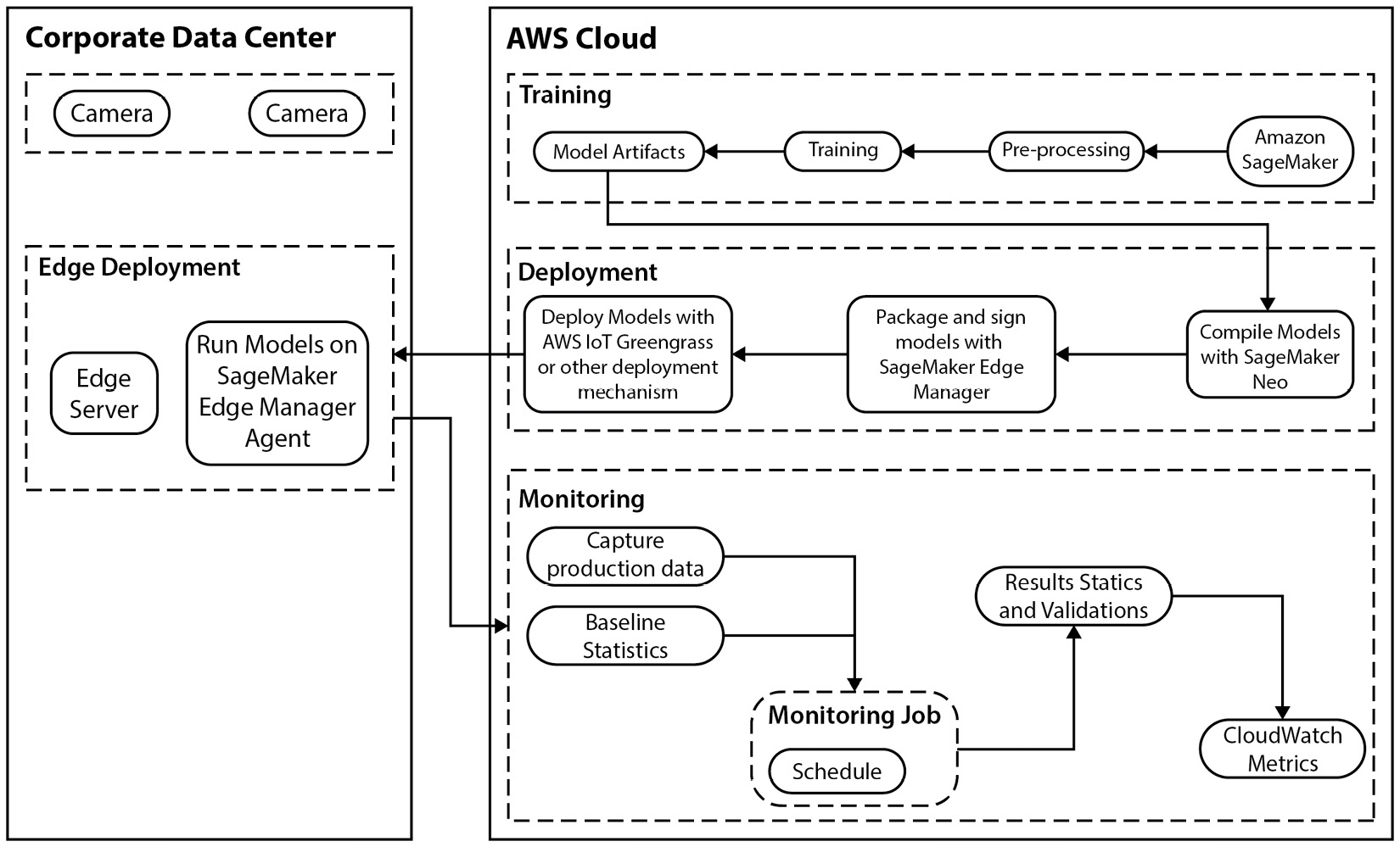
Figure 8.1 – Architecture for edge deployments using Amazon SageMaker and IoT Greengrass
As you can see from Figure 8.1, a typical architecture is divided into two separate and individual architectures. One for the cloud-based components and one for the edge components. At a high level, the cloud environment is used to build, deploy, and manage the use case application being deployed to the edge. The corresponding edge environment, or the corporate data center, in this case, is where the edge devices reside, and in turn, execute upon the ML use case by running the supported ML models. From an ML use case perspective, Figure 8.1 also shows the cameras attached to the edge server device, allowing any video captured to be streamed to the ML model in order for the model to classify the objects detected in the video frames. Figure 8.1 shows a simplistic flow for the CV use case, from training an ML model on SageMaker to deploying it to the edge server using Greengrass, and then managing and monitoring the solution. But building out the actual solution is very complicated.
So, to illustrate this complexity, in the next section, we are going to build out this architecture by breaking out each component, starting with the corporate data center or edge architecture.
Building the edge components
As highlighted in the previous section, the corporate data center serves as the edge location for our CV use case. Inside this edge location, we have a number of cameras, connected to a compute device, or edge server, that runs the CV model. Since we don’t have access to a corporate data center, within the context of the book, we will simulate building out the edge environment using an Elastic Compute Cloud (EC2) instance.
Note
If you are not accustomed to working with EC2 instances, you can familiarize yourself with them by referencing the following documentation: https://aws.amazon.com/ec2/getting-started/.
The following steps will demonstrate how to set up the edge server using an EC2 instance and configure the necessary Greengrass software as well as the required security permissions. Let’s get started with setting up the appropriate Identity and Access Management (IAM) roles and permissions:
- Log into your AWS account and open the IAM console (https://console.aws.amazon.com/iam/home).
- Once the IAM console is open, use the left-hand navigation panel and click on Roles to open the Roles dashboard. Then click on the Create role button in the top-right corner.
- Once the Create role wizard starts, select AWS Service as the Trusted entity type.
- For the Use case, select EC2 and click on the Next button.
- On the Add permissions page, click on the Create policy button in the top right to open the Create policy page.
- On the Create policy page, select the JSON tab, paste the policy from the SageMakerGreenGrassV2MinimalResourcePolicy.json file in GitHub (https://github.com/PacktPublishing/Applied-Machine-Learning-and-High-Performance-Computing-on-AWS/blob/main/Chapter08/SageMakerGreenGrassV2MinimalResourcePolicy.json), and make sure to update the <account_id> tag in the policy with your AWS account ID.
- Click on the Next: Tags button.
- Click on the Next: Review button.
- On the Review policy page, name the policy SageMakerGreenGrassV2MinimalResourcePolicy, and click the Create policy button.
- Go back to the Add permission page from step 5, and refresh the page to capture the newly created IAM policy.
- Search for the SageMakerGreenGrassV2MinimalResourcePolicy policy in the search bar, and once found, select the checkbox for the policy to add the permission, then click the Next button.
- On the Role details page, enter SageMakerGreenGrassV2MinimalResourceRole, as the Role name.
- Once again, using the Role dashboard, click the newly created SageMakerGreenGrassV2MinimalResourceRole role to open the Role summary page.
- Now, click the Add permissions dropdown and select the Attach policies option.
- Search for the AmazonSageMakerEdgeDeviceFleetPolicy policy, and click on the checkbox to select this policy.
- Repeat the process shown in step 15, except this time, select the checkbox for the AmazonSageMakerFullAccess, AWSIoTLogging, AmazonS3FullAccess, AWSIoTRuleActions, AWSIoTThingsRegistration, and AmazonSSMManagedInstanceCore policies.
- With these policies selected, click the Attach policies button.
- In the Role summary page from step 13, click the Add permissions dropdown and select the Create inline policy option.
- On the Create policy page, click the JSON tab and add the following policy statement:
{"Version":"2012-10-17",
"Statement":[
{"Sid":"GreengrassComponentAccess",
"Effect":"Allow",
"Action":[
"greengrass:CreateComponentVersion",
"greengrass:DescribeComponent"
],
"Resource":"*"
}
]
}
- Click the Review policy button.
- Name the policy GreengrassComponentAccessPolicy and click the Create policy button.
- In the Role summary page, click the Trust relationships tab and click the Edit trust policy button.
- Replace the existing policy with the following trust policy statement:
{"Version": "2012-10-17",
"Statement": [
{"Effect": "Allow",
"Principal": {"Service": "ec2.amazonaws.com"
},
"Action": "sts:AssumeRole"
},
{"Effect": "Allow",
"Principal": {"Service": "credentials.iot.amazonaws.com"
},
"Action": "sts:AssumeRole"
},
{"Effect": "Allow",
"Principal": {"Service": "sagemaker.amazonaws.com"
},
"Action": "sts:AssumeRole"
}
]
}
Now that we have set up the necessary permissions, next we can configure the edge server with the following steps showing us how to configure the EC2 instance:
- Before creating the EC2 instance, we need to configure the necessary scripts that customize the EC2 instance as an edge server. To provide easy command line access to AWS resources, open the AWS CloudShell console (https://console.aws.amazon.com/cloudshell/home).
- Once the CloudShell console has been initialized in the browser, clone the companion GitHub repository by running the following command:
$ git clone https://github.com/PacktPublishing/Applied-Machine-Learning-and-High-Performance-Computing-on-AWS src && cd src/Chapter08
- Next, we create an S3 bucket and store the configuration scripts for the EC2 instance by running the following commands:
$ export AWS_ACCOUNT=$(aws sts get-caller-identity --query "Account" --output text)
$ aws s3 mb s3://ec2-scripts-$AWS_REGION-$AWS_ACCOUNT
$ aws s3 sync scripts s3://ec2-scripts-$AWS_REGION-$AWS_ACCOUNT/scripts
- Run the following command to capture the name of the S3 bucket containing the EC2 configuration scripts:
$ echo ec2-scripts-$AWS_REGION-$AWS_ACCOUNT
Note
Make sure to remember the name of the S3 bucket containing the EC2 instance configuration scripts, as it will be used in a later step.
- Open the EC2 management console (https://console.aws.amazon.com/ec2/v2/home) in a browser tab.
- Once the EC2 console is open, click the Launch instance button.
- In the Launch an instance wizard, in the Name and tags section, enter edge-server as the name for this instance.
- Select AMI as amzn2-ami-kernel-5.10-hvm-2.0.20220426.0-x86_64-gp2 and instance type as c5.large.
- Scroll down to the Configure storage section and specify 20 GiB for Root volume.
- Using the IAM instance profile drop-down box in the Advance details section, select the SageMakerGreenGrassV2MinimalResourceRole role.
- In the User data text box of the Advance details section, paste the following Bash code:
#!/bin/bash
aws s3 cp s3://<REPLACE WITH THE NAME OF YOUR S3 BUCKET>/scripts/ /home/ec2-user --recursive
sleep 30
process_id=$!
wait $process_id
sudo yum update -y
sudo yum install docker -y
sudo yum install python-pip -y
sudo pip3 install boto3
sudo pip3 install requests
cd /home/ec2-user
python3 getResourceTempCredentials.py
sudo service docker start
sudo usermod -a -G docker ec2-user
docker build -t "aws-iot-greensgrass:2.5" ./
chmod +x dockerRun.sh
Note
Make sure to replace the S3 bucket name with the name of your S3 bucket from the output of step 4.
- Click the Launch instance button to create the EC2 instance.
- Wait 10 minutes after the EC2 instance is in the active state before logging in to the EC2 instance, as the Bash script in the user data will need some time to install the necessary packages and build the Docker image for AWS IoT Greengrass software.
- Log into the EC2 instance, and ensure you are in the /home/ec2-user directory. Using vi, open the env file, and ensure the AWS_REGION variable is set to the current AWS Region being used. For example, the following output shows the env file configured for the us-east-1 Region:
GGC_ROOT_PATH=/greengrass/v2
AWS_REGION=us-east-1
PROVISION=true
THING_NAME=mything
THING_GROUP_NAME=mythinggroupname
TES_ROLE_NAME=GreengrassV2TokenExchangeRole
TES_ROLE_ALIAS_NAME=GreengrassCoreTokenExchangeRoleAlias
COMPONENT_DEFAULT_USER=ggc_user:ggc_group
DEPLOY_DEV_TOOLS=true
Note
You can also customize the THING_NAME and THING_GROUP_NAME parameters. However, make sure these variables are in lowercase.
- Save and exit the env file.
- Run the Docker container by executing the following command:
$ ./dockerRun.sh
Note
In case you need to restart the Greengrass V2 Docker container, make sure to get the new credentials by running the following command:
$ rm credentials #remove the old credentials file
$ sudo python3 getResourceTempCredentials.py # create credentials file with new credentials
$ ./dockerRun.sh
- Open another terminal window, log in to the EC2 instance, and run the following command to verify that Greengrass V2 is running and retrieve the container ID:
$ docker ps
- You can then run the following command to access the container and explore the AWS IoT Greengrass Core software running inside the container:
$ docker exec -it container-id /bin/bash
Note
When you use docker exec to run commands inside the Docker container, these are not captured in the Docker logs. As a best practice, we recommend you log your commands in the Docker logs so that you can look into the state of the Greengrass Docker container in case you need to troubleshoot any issues.
- Run the following command in a different terminal. It will attach your terminal’s input, output, and error to the container running currently. This will help you to view and control the container from your terminal.
$ docker attach container-id
By executing these steps, we have effectively configured an EC2 instance to run our ML model as an edge server. So, with the edge components of our architecture successfully built, we can move on to building the ML model.
Building the ML model
Building the ML model involves training an optimal ML model to suit our business use case. As we’ve seen in previous chapters, Amazon SageMaker provides us with distinct capabilities that allow us to ingest and process the necessary training data, as well as train and optimize the best ML model. Additionally, we saw that SageMaker also allows us to deploy and host these models in the cloud, and as we will see, SageMaker also allows us to deploy and manage ML models at the edge.
The following steps will walk you through how to build an ML model that suits our use case, compile the model for an edge environment, and then deploy the model to the edge, all using SageMaker:
- Within your AWS account, open the Amazon SageMaker management console (https://console.aws.amazon.com/sagemaker/home).
- Launch the SageMaker Studio IDE.
Note
For more information on how to create and launch the SageMaker Studio IDE, please refer to the Setting up EMR and SageMaker Studio section of Chapter 5, Data Analysis.
- Once the SageMaker Studio IDE has launched, use the File Browser navigation panel and double-click on the cloned Applied-Machine-Learning-and-High-Performance-Computing-on-AWS folder to expand it.
- Then, double-click on the Chapter_8 folder to open it for browsing.
- Double-click on the sagemaker_notebook folder, and then launch the 1_compile_resnet_model_egde_manager.ipynb notebook.
- Once the notebook has started, use the menu bar to select the Kernel menu and then the Restart Kernel and Run All Cells… option.
Once the notebook has run, we will have our image classification model running on the edge server and managed as part of a fleet. Nonetheless, let’s verify this by reviewing some of the important code cells in the notebook. The first part of the notebook downloads an already optimized or pre-trained ResNet-18 (https://arxiv.org/pdf/1512.03385.pdf) model. This is essentially our optimized ML for the image classification use case that we have deployed to the edge. After setting up the SageMaker environment variables and establishing the necessary permissions, we upload the pre-trained model to S3. Once the model has been stored in the cloud, and as you can see from the following code snippet, we instantiate the pre-trained ResNet-18 model as a PyTorch-based SageMaker model object called sagemaker_model:
from sagemaker.pytorch.model import PyTorchModel
from sagemaker.predictor import Predictor
sagemaker_model = PyTorchModel(
    model_data=model_uri,
    predictor_cls=Predictor,
    framework_version=framework_version,
    role=role,
    sagemaker_session=sagemaker_session,
    entry_point="inference.py",
    source_dir="code",
    py_version="py3",
    env={"MMS_DEFAULT_RESPONSE_TIMEOUT": "500"},
)
With the model object defined, we then use SageMaker Neo (https://docs.aws.amazon.com/sagemaker/latest/dg/neo.html) to compile a model that suites the specific compute architecture of the edge device, in this case, our X86_64 Linux edge server:
sagemaker_client = boto3.client("sagemaker", region_name=region)
target_arch = "X86_64"
target_os = 'LINUX'
response = sagemaker_client.create_compilation_job(
    CompilationJobName=compilation_job_name,
    RoleArn=role,
    InputConfig={
        "S3Uri": sagemaker_model.model_data,
        "DataInputConfig": data_shape,
        "Framework": framework,
    },
    OutputConfig={
        "S3OutputLocation": compiled_model_path,
#         "TargetDevice": 'jetson_nano',
        "TargetPlatform": {
            "Arch": target_arch,
            "Os": target_os
        },
    },
    StoppingCondition={"MaxRuntimeInSeconds": 900},
)
Note
Make sure to take note of the S3 path for the compiled model, as we will be using this path to deploy the model package.
After compiling the model for the edge server, we verify the model’s functionality by deploying it as a SageMaker-hosted endpoint, and then using the following code to generate a sample inference for a test image:
import numpy as np
import json
with open("horse_cart.jpg", "rb") as f:
    payload = f.read()
    payload = bytearray(payload)
response = runtime.invoke_endpoint(
    EndpointName=ENDPOINT_NAME,
    ContentType='application/octet-stream',
    Body=payload,
    Accept = 'application/json')
result = response['Body'].read()
result = json.loads(result)
print(result)
Once we’ve verified that the model functions correctly, essentially being able to classify the image correctly, we can then package the model as shown in the following code snippet:
packaging_job_name = compilation_job_name + "-packaging-ggv2"
component_name = "SagemakerEdgeManager" + packaging_job_name
response = sagemaker_client.create_edge_packaging_job(
    RoleArn=role,
    OutputConfig={
        "S3OutputLocation": s3_edge_output_location,
    },
    ModelName=packaged_model_name,
    ModelVersion=model_version,
    EdgePackagingJobName=packaging_job_name,
    CompilationJobName=compilation_job_name,
)
Finally, once the model has been packaged, we can use the create_device_fleet() method to create a manageable fleet of edge devices to host the newly compiled ML model and then use the register_device() method to initialize our EC2 edge server as a registered or managed edge device that runs our ML model:
s3_device_fleet_output = os.path.join(s3_edge_output_location, 'fleet')
iot_role_arn = f'arn:aws:iam::{account_id}:role/SageMakerGreenGrassV2MinimalResourceRole'
device_fleet_name = "mydevicefleet"
device_name = 'mything'
sagemaker_client.create_device_fleet(
    DeviceFleetName=device_fleet_name,
    RoleArn=iot_role_arn, # IoT Role ARN specified in previous step
    OutputConfig={
        'S3OutputLocation': s3_device_fleet_output
    }
)
sagemaker_client.register_devices(
    DeviceFleetName=device_fleet_name,
    Devices=[
        {
            "DeviceName": device_name,
            "IotThingName": device_name
        }
    ]
)
Once the model has been trained and compiled and the edge server registered as a SageMaker-managed edge device, we can go ahead and deploy the model package to the edge server.
Deploying the model package
To deploy the model package to the edge server, we will register it as a Greengrass component and then deploy the component to the edge server using the Greengrass console. The following steps will walk us through how to do this:
- Using a web browser, open the AWS IoT management console (https://console.aws.amazon.com/iot/home).
- In the Manage section of the left-hand navigation panel, expand the Greengrass devices option and click on Components.
- Click on the Create component button.
- After the Create component page loads, ensure that the Enter recipe as JSON option is selected, and paste the com.greengrass.SageMakerEdgeManager.ImageClassification.Model.json file contents into the Recipe box.
Note
The com.greengrass.SageMakerEdgeManager.ImageClassification.Model.json file can be found in the companion GitHub repository (https://github.com/PacktPublishing/Applied-Machine-Learning-and-High-Performance-Computing-on-AWS/blob/main/Chapter08/custom_component_recipes/com.greengrass.SageMakerEdgeManager.ImageClassification.Model.json).
- Update the S3 location of the packaged model under the Artifacts tag of the JSON file to match the S3 path for the compiled model.
Note
The S3 location of the packaged model is the output from the create_compilation_job() method used in the previous section.
- Click on the Create component button.
- Go to your S3 bucket and create the artifacts folder, and inside it, create another folder with the name com.greengrass.SageMakerEdgeManager.ImageClassification. Your S3 path should look like this: s3://<bucket_name>/artifacts/com.greengrass.SageMakerEdgeManager.ImageClassification/.
- Upload the image_classification.zip and installer.sh files from the GitHub repo (https://github.com/PacktPublishing/Applied-Machine-Learning-and-High-Performance-Computing-on-AWS/tree/main/Chapter08) to the S3 location defined in step 7.
- Update the S3 location of the image_classification.zip and installer.sh files under the Artifacts tag of the JSON file to match the S3 path defined in step 8.
- Repeat step 3 and step 4 for the com.greengrass.SageMakerEdgeManager.ImageClassification component.
Note
The com.greengrass.SageMakerEdgeManager.ImageClassification.json file can be found in the companion GitHub repository (https://github.com/PacktPublishing/Applied-Machine-Learning-and-High-Performance-Computing-on-AWS/blob/main/Chapter08/custom_component_recipes/com.greengrass.SageMakerEdgeManager.ImageClassification.json).
With the Greengrass components registered, we can now deploy them to the edge server and run image classification inference using the components that we just created. Deploying these components downloads a SageMaker Neo-compiled pre-trained ML model and installs the SageMaker Edge Manager agent on the edge server. However, before we can actually perform the deployment of these components, we have to subscribe to the notification topic in order to view and manage any inference tasks on the edge server. The following steps will walk us through how to subscribe to a topic:
- Go to the AWS IoT console (https://console.aws.amazon.com/iot/) and click on MQTT test client from the Test option of the left-hand navigation panel.
- In the Topic name box of the Subscribe to a topic tab, enter gg/sageMakerEdgeManager/image-classification.
- Click the Subscribe button.
With the ability to monitor and manage any inference requests to the ML model running on the edge server in place, we can deploy the Greengrass components. The following steps will show us how to do this (they are also highlighted in the AWS Greengrass Developer guide at https://docs.aws.amazon.com/greengrass/v2/developerguide/greengrass-v2-developer-guide.pdf):
- In the AWS IoT Greengrass console (https://console.aws.amazon.com/greengrass) navigation menu, choose Deployments, and then choose the deployment for the target device.
- On the deployment page, choose Revise and then choose Revise deployment.
- On the Specify target page, click Next.
- Under the My components option of the Select components page, select both the com.greengrass.SageMakerEdgeManager.ImageClassification, and com.greengrass.SageMakerEdgeManager.ImageClassification.Model components.
- Under Public components, turn off the Show only selected components toggle, and then select the aws.greengrass.SageMakerEdgeManager component.
- Click Next.
- On the Configure components page, select the aws.greengrass.SageMakerEdgeManager component, and choose Configure component.
- Under Configuration update, in Configuration to merge, enter the following configuration:
{"DeviceFleetName": "device-fleet-name",
"BucketName": "S3-BUCKET"
}
Note
Replace device-fleet-name and the S3 bucket name with the corresponding values you created when creating the device fleet in the notebook.
- Choose Confirm, and then choose Next.
- On the Configure advanced settings page, keep the default configuration settings and choose Next.
- On the Review page, choose Deploy.
The deployment can take several minutes to complete. After the components have been deployed, we can view, manage, and monitor the ML model inference results in the component log of the Greengrass Core device, as well as in the AWS IoT MQTT client of the AWS IoT console. To view the inference results in the component log of the Greengrass Core device, log into the edge server EC2 instance and run the following command:
$ sudo tail –f /greengrass/v2/logs/com.greengrass.SageMakerEdgeManager.ImageClassification.log
You should see Top 5 predictions with score 0.3 or above in the logs similar to the one shown here:
2022-08-15T03:38:45.437Z [INFO] (Copier) com.greengrass.SageMakerEdgeManager.ImageClassification: stdout. {"timestamp": "2022-08-15 03:38:45.282879+00:00", "inference-type": "image-classification", "inference-description": "Top 5 predictions with score 0.3 or above ", "inference-results": [{"Label": "slot, one-armed bandit", "Score": "83.41295623779297"}, {"Label": "mousetrap", "Score": "75.826416015625"}, {"Label": "comic book", "Score": "73.64051055908203"}, {"Label": "microphone, mike", "Score": "71.14073181152344"}, {"Label": "honeycomb", "Score": "68.3149185180664"}]}. {scriptName=services.com.greengrass.SageMakerEdgeManager.ImageClassification.lifecycle.run.script, serviceName=com.greengrass.SageMakerEdgeManager.ImageClassification, currentState=RUNNING}Alternatively, you can also view the results in MQTT test client on the AWS IoT console (https://console.aws.amazon.com/iot/) by clicking MQTT test client from the Test option on the left-hand navigation panel. In the Subscriptions section, you will see the prediction results, as shown in the following screenshot:

Figure 8.2 – Inference results on MQTT test client on AWS IoT console
If you can’t see inference results in the MQTT client, the deployment might have failed or it did not reach the core device. This can occur primarily due to two reasons: your core device is not connected to the network, or it doesn’t have the right permissions to execute the component. To troubleshoot it, you can run the following command on your core device. This command will open the AWS IoT Greengrass Core software log file, which includes logs from the Greengrass Core device’s deployment service.
$ sudo tail -f /greengrass/v2/logs/greengrass.log
Note
For more information, see the troubleshooting documentation: https://docs.aws.amazon.com/greengrass/v2/developerguide/ml-troubleshooting.html.
With the Greengrass components now deployed to the edge server, we have successfully deployed our ML model to the edge. Furthermore, by leveraging the capabilities of AWS IoT Greengrass, as well as Amazon SageMaker, we have not only compiled the ML to function efficiently and ensure performance on the edge device but also established a mechanism to manage and monitor the environment. As you will recall from the Reviewing the key considerations for optimal edge deployments section, these are the key factors that make up an optimal edge architecture.
Summary
In this chapter, we introduced you to the concept of deploying ML models outside of the cloud, primarily on an edge architecture. To lay the foundation for how to accomplish an edge deployment, we also examined what an edge architecture is, as well as the most important factors that need to be considered when designing an edge architecture, namely efficiency, performance, and reliability.
With these factors in mind, we explored how the AWS IoT Greengrass, as well as Amazon SageMaker services, can be used to build an optimal ML model package in the cloud, compiled to run efficiently on an edge device, and then deployed to the edge environment, in a reliable manner. In doing so, we also highlighted just how crucial the ability to manage and monitor both the edge devices, as well as the deployed ML models is to create an optimal edge architecture.
In the next chapter, we will continue along the lines of performance monitoring and optimization of deployed ML models.