7

Deploying Machine Learning Models at Scale

In previous chapters, we learned about how to store data, carry out data processing, and perform model training for machine learning applications. After training a machine learning model and validating it using a test dataset, the next task is generally to perform inference on new and unseen data. It is important for any machine learning application that the trained model should generalize well for unseen data to avoid overfitting. In addition, for real-time applications, the model should be able to carry out inference with minimal latency while accessing all the relevant data (both new and stored) needed for the model to do inference. Also, the compute resources associated with the model should be able to scale up or down depending on the number of inference requests, in order to optimize cost while not sacrificing performance and inference requirements for real-time machine learning applications.

For use cases that do not require real-time inference, the trained model should be able to carry out inference on very large datasets with thousands of variables in a reasonable amount of time as well. In addition, in several scenarios, we may not want to go through the effort of managing servers and software packages needed for inference, and instead, focus our effort on developing and improving our machine learning models.

Keeping all these aforementioned factors in mind, AWS provides multiple options for deploying machine learning models to carry out inference on new and unseen data. These options consist of real-time inference, batch inference, and asynchronous inference. In this chapter, we are going to discuss the managed deployment options of machine learning models using Amazon SageMaker, along with various features such as high availability of models, auto-scaling, and blue/green deployments.

We will cover the following topics in this chapter:

• Managed deployment on AWS
• Choosing the right deployment option
• Batch inference
• Real-time inference
• Asynchronous inference
• High availability of model endpoints
• Blue/green deployments

Managed deployment on AWS

Data scientists and machine learning practitioners working on developing machine learning models to solve business problems are often very focused on model development. Problem formulation and developing an elegant solution, choosing the right algorithm, and training the model so that it provides reliable and accurate results are the main components of the machine learning problem solving cycle that we want our data scientists and data engineers to focus on.

However, once we have a good model, we want to run real-time or batch inference on new data. Deploying the model and then managing it are tasks that often require dedicated engineers and computation resources. This is because, we first need to make sure that we have all the right packages and libraries for the model to work correctly. Then, we also need to decide on the type and amount of compute resources needed for the model to run. In real-time applications, we often end up designing for peak performance requirements, just like provisioning servers for IT projects.

After the model is deployed and is running, we also need to make sure that everything stays working in the manner that we expect it to. Furthermore, in real world scenarios, data scientists often have to manually carry out analysis periodically to detect model or data drift. In the event that either of these drifts are detected, the data scientists go through the entire cycle of exploratory analysis, feature engineering, model development, model training, hyperparameter optimization, model evaluation, and model deployment again. All these tasks consume a lot of effort and resources and due to this reason, many organizations have moved to automating these processes using machine learning operations (MLOps) workflows and managed model deployment options that scale well with varying workloads.

Amazon SageMaker offers multiple fully managed model deployment options. In this section, we give an overview of these managed deployment options along with their benefits and then discuss a few of these deployment options in detail in the following sections.

Amazon SageMaker managed model deployment options

Amazon SageMaker offers the following managed deployment model options:

• Batch Transform: SageMaker Batch Transform is used to carry out inference on large datasets. There is no persistent endpoint in this case. This method is commonly used to carry out inference in a non-real-time machine learning use case requiring offline inference on larger datasets.
• Real-time endpoint: A SageMaker real-time endpoint is for use cases where a persistent machine learning model endpoint is needed, which carries out inference on a few data samples in real time.
• Asynchronous inference: Amazon SageMaker Asynchronous Inference deploys an asynchronous endpoint for carrying out inference on large payloads (up to 1 GB) with large processing times and low latency.
• Serverless Inference: In all the previous methods, the user is required to select the compute instance types for inference. Amazon SageMaker Serverless Inference automatically chooses the server type and scales up and down based on the load on the endpoint. It is often useful for applications that have unpredictable traffic patterns.

Let’s explore the variety of available compute resources next.

The variety of compute resources available

To carry out inference, there are a wide variety of computation instances available. At the time of writing, approximately 70+ instances are available for carrying out machine learning inference. These instances have varying levels of computation power and memory available to serve different use cases. There is also the option of using graphical processing units (GPUs) for inference. In addition, SageMaker also supports Inf1 instances for high-performance and low-cost inference. These options make SageMaker model deployment and inference highly versatile and suitable for a variety of machine learning use cases.

Cost-effective model deployment

Amazon SageMaker has various options for optimizing model deployment cost. There are multi-model endpoints, where multiple models can share a container. This helps with reducing hosting costs since endpoint utilization is increased due to multiple models sharing the same endpoint. In addition, it also enables time sharing of memory resources across different models. SageMaker also has the option of building and deploying multi-container endpoints. Furthermore, we can attach scaling policies to our endpoints to allocate more compute resources when traffic increases, and shut down instances when traffic decreases in order to save on costs.

Another cost-effective option for model deployment is SageMaker Serverless Inference. Serverless Inference utilizes AWS Lambda to scale up and down compute resources as traffic increases or decreases. It is especially useful for scenarios with unpredictable traffic patterns.

Blue/green deployments

SageMaker automatically uses blue/green deployment whenever we update a SageMaker model endpoint. In blue/green deployment, SageMaker uses a new fleet of instances to deploy the updated endpoints and then shifts the traffic to the updated endpoint from the old fleet to the new one. Amazon SageMaker offers the following traffic-shifting strategies for blue/green deployments:

• All at once traffic shifting
• Canary traffic shifting
• Linear traffic shifting

We will discuss these traffic patterns in more detail later in this chapter.

Inference recommender

With Amazon SageMaker Inference Recommender, we can automatically get recommendations on the type of compute instance to use for deploying our model endpoint. It gives us instance recommendations by load testing various instances and outputs inference costs, along with throughput and latency, for the tested instance types. This helps us decide on the type of instance to use for deploying our model endpoint.

MLOps integration

Using Amazon SageMaker, we can easily build machine learning workflows that integrate with continuous integration and continuous delivery (CI/CD) pipelines. These workflows can be used to automate the entire machine learning life cycle, including data labeling, data processing and feature engineering, model training and registry, post-processing, endpoint deployment, and model monitoring for data and model drift monitoring. For model deployment, these workflows can be used to automate the process of doing batch inference, as well as pushing model endpoints from development to staging to production environments.

Model registry

Amazon SageMaker provides the capability to register and catalog machine learning models with the SageMaker model registry. Using the model registry, we can include different versions of a trained model in a model package group. This way, whenever we train and register a model, it is added as a new version to the model package group. In addition, using the model registry, we can also associate metadata and training metrics to a machine learning model, approve or reject a model, and if approved, move the models to production. These features of the model registry facilitate the building of CI/CD pipelines needed for automating machine learning workflows.

Elastic inference

For machine learning use cases that require very high throughput and low latency, we often end up using GPU machines, thereby increasing the cost of inference significantly. Using Amazon SageMaker, we can add elastic inference to our endpoints. Elastic inference provides inference acceleration to our endpoint, by attaching just the right amount of GPU-powered inference acceleration to any SageMaker instance type. This helps significantly with latency and throughput, while also achieving it at a much lower cost compared to using GPU instances for inference.

Deployment on edge devices

Many machine learning use cases require models to run on edge devices such as mobile devices, cameras, and specialized devices. These devices often have low compute resources, memory, and storage. Furthermore, deploying, managing, and monitoring machine learning models on a fleet of devices is a difficult task because of the variability in device hardware and operating systems. With Amazon SageMaker Edge Manager, machine learning models can be deployed, monitored, and managed on a fleet of devices with different hardware and software configurations. SageMaker Edge Manager uses SageMaker Neo to compile machine learning models and packages these compiled models to be deployed on edge devices. In addition, we can also sample the data used by the model on the edge devices and send them to the cloud to carry out analysis to determine quality issues such as data and model drift.

Now, let’s discuss the various model deployment options on AWS in the following section.

Choosing the right deployment option

As mentioned in the previous section, AWS has multiple model deployment and inference options. It can get confusing and overwhelming sometimes to decide on the right option for model deployment. The decision to select the right model deployment option really depends on the use case parameters and requirements. A few important factors to consider while deciding on deployment options are listed as follows:

• Do we have an application that needs a real-time, persistent endpoint to carry out on-demand inference on new data in real time and very quickly with low latency and high availability?
• Can our application wait for a minute or two for the compute resources to come online before getting the inference results?
• Do we have a use case where we do not need results in near real time? Can we do inference on a batch of data once a day/week or on an as-needed basis?
• Do we have an unpredictable and non-uniform traffic pattern requiring inference? Do we need to scale up and down our compute resources based on the traffic?
• How big is the data (number of data points/rows) that we are trying to do inference on?
• Do we need dedicated resources all the time to carry out inference or can we follow a serverless approach?
• Can we pack in multiple models in a single endpoint to save on cost?
• Do we need to have an inference pipeline consisting of multiple models, pre-processing steps, and post-processing steps?

In the following subsections, we will discuss when to pick the different types of model deployment and inference options provided by Amazon SageMaker, while addressing the previously mentioned questions. We will also provide examples of typical example use cases for each of the model deployment options.

Using batch inference

Amazon SageMaker Batch Transform is used when there is no need for a persistent, real-time endpoint and inference can be done on large batches of data. The following examples illustrate the use of SageMaker Batch Transform:

• Predictive maintenance: In a manufacturing plant, sensor and machine data for various components could be collected the entire day. For such a use case, there is no need for real-time or asynchronous endpoints. At night, machine learning models can be used for predicting whether a component is about to fail, or whether a part of the machinery needs maintenance. These models would run on large batches of data and carry out inference using SageMaker Batch Transform. The results from these models could then be used to make and execute a maintenance schedule.
• Home prices prediction: Real estate companies collect data for a few days (and sometimes weeks) before coming out with new home prices and market direction predictions. These models do not need real-time or asynchronous endpoints as they need to be run only after a few days or weeks and on large amounts of data. For such use cases, SageMaker Batch Transform is the ideal option for inference. SageMaker Batch Transform jobs could run on a fixed interval in a machine learning pipeline on new and historical data, carrying out inference to predict home price adjustments and market direction by localities. These results can, in turn, then be used to determine if the machine learning models need to be retrained.

We will cover batch, real-time, and asynchronous inference options in Amazon SageMaker in detail in the later sections of this chapter.

Using real-time endpoints

Amazon SageMaker real-time endpoints should be the choice for model deployment when there is a need for a real-time persistent model endpoint, doing predictions with low latency as new data arrives. Real-time endpoints are fully managed by Amazon SageMaker and can be deployed as multi-model and multi-container endpoints. The following are some example use cases for real-time endpoints:

• Fraudulent transaction: A customer uses a credit card to purchase an item online or physically in a retail store. This financial transaction can be carried out by the actual owner of the credit card or it can be a stolen credit card as well. The financial institution needs to make the decision in real time whether to approve the transaction or not. In such a scenario, a machine learning model can be deployed as a real-time endpoint. This model could use customer’s demographic data and history of purchases from historical data tables, while also using some data from the current transaction, such as IP address and web browser parameters (if it is an online transaction), or store location and image and/or video from a camera in real time (if it is a physical transaction), to classify whether the transaction is fraudulent or not. This decision can then be used by the financial institution to either approve or reject the transaction, or contact the customer for notification, manual authentication, and approval.
• Real-time sentiment analysis: A customer is having a chat or phone conversation with a customer care agent. A machine learning model is analyzing the chat or transcribed text from voice conversation in real time to decide on the sentiment that the customer is showing. Based on the sentiment, if the customer is unhappy, the agent can offer various promotions or escalate the case to a supervisor before things get out of hand. This machine learning model should be deployed using a real-time endpoint so that the sentiment can be correctly determined without any lag or delay.
• Quality assurance: In a manufacturing plant, products are being assembled on an assembly line and there needs to be strict quality control to remove defective products as soon as possible. This is again an application where real-time inference from a machine learning model classifying the objects as defective or normal using live images or video feed will be useful.

Similar to real-time endpoints, we also have the option of using asynchronous endpoints, which we will learn about in the following section.

Using asynchronous inference

Amazon SageMaker Asynchronous Inference endpoints are very similar to real-time endpoints. Asynchronous endpoints can queue inference requests and are the deployment option of choice when near real-time latency is needed, while also processing large workloads. The following example illustrates a potential asynchronous endpoints use case.

Train track inspection: Several trains are running on their everyday routes with attached cameras that take images and videos of train tracks and switches for defect detection. These trains do not have a high bandwidth available to transmit this data in real time for inference. When these trains dock at a station, a large number of images and videos could be sent to a SageMaker Asynchronous Inference endpoint for inference to find out whether everything is normal, or if there are any defects present anywhere on the track or switches. The compute instance associated with the asynchronous endpoint will start as soon as it receives data from any of the trains, carrying out inference on the data, then shutting down once all the data has been processed. This will help with the reduction in costs compared to a real-time endpoint.

Batch inference

For carrying out batch inference on datasets, we can use SageMaker Batch Transform. It should be used for inference when there is no need for a real-time persistent deployed machine learning model. Batch Transform is also useful when the dataset for inference is large or if we need to carry out heavy preprocessing on the dataset. For example, removing bias or noise from the data, converting speech data to text, and filtering and normalization of images and video data.

We can pass input data to SageMaker Batch Transform in either one file or using multiple files. For tabular data in one file, each row in the file is interpreted as one data record. If we have selected more than one instance for carrying out the batch transform job, SageMaker distributes the input files to different instances for batch transform jobs. Individual data files can also be split into multiple mini-batches and batch transform on can be carried out these mini-batches in parallel on separate instances. Figure 7.1 shows a simplified typical architecture example of SageMaker Batch Transform:

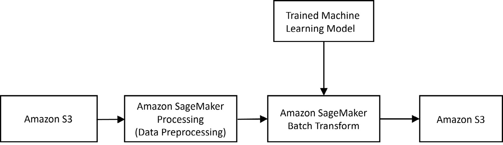
Figure 7.1 – Example architecture for Amazon SageMaker Batch Transform

As shown in the figure, data is read from Amazon S3. Preprocessing and feature engineering is carried out on this data using Amazon SageMaker Processing in order to transform the data in the right format that the machine learning model expects. A trained machine learning model is then used by Amazon SageMaker Batch Transform to carry out batch inference. The results are then written back to Amazon S3. The machine learning model used by Batch Transform could either be trained using Amazon SageMaker or can be a model trained outside of Amazon SageMaker. The two main steps in Batch Transform are as follows:

1. Creating a transformer object.
2. Creating a batch transform job for carrying out inference.

These steps are described in the following subsections.

Creating a transformer object

We first need to create an object of the Transformer class in order to run a SageMaker batch transform job. While creating the Transformer object, we can specify the following parameters:

• model_name: This is the name of the machine learning model that we are going to use for inference. This can also be a built-in SageMaker model, for which we can directly use the transformer method of the built-in estimator.
• instance_count: The number of EC2 instances that we are going to use to run our batch transform job.
• instance_type: The type of EC2 instances that we can use. A large variety of instances are available to be used for batch transform jobs. The choice of instance depends on our use case’s compute and memory requirements, as well as the data type and size.

In addition, we can also specify several other parameters such as batch strategy, and output path. The complete list of parameters can be found on the documentation page in the References section. In the following example, we used SageMaker’s built-in XGBoost container. For running batch transformers for your own containers/models or frameworks, such as PyTorch and TensorFlow, the container images may vary.

Figures 7.2 – 7.8 show an example of SageMaker’s XGBoost model being fit on our training data and then a transformer object being created for this training model. We specified that the transform job should run on one instance of type ml.m4.xlarge and should expect text/csv data:

1. As shown in Figure 7.2, we can specify the various packages and SageMaker parameters needed to run the code in the example.

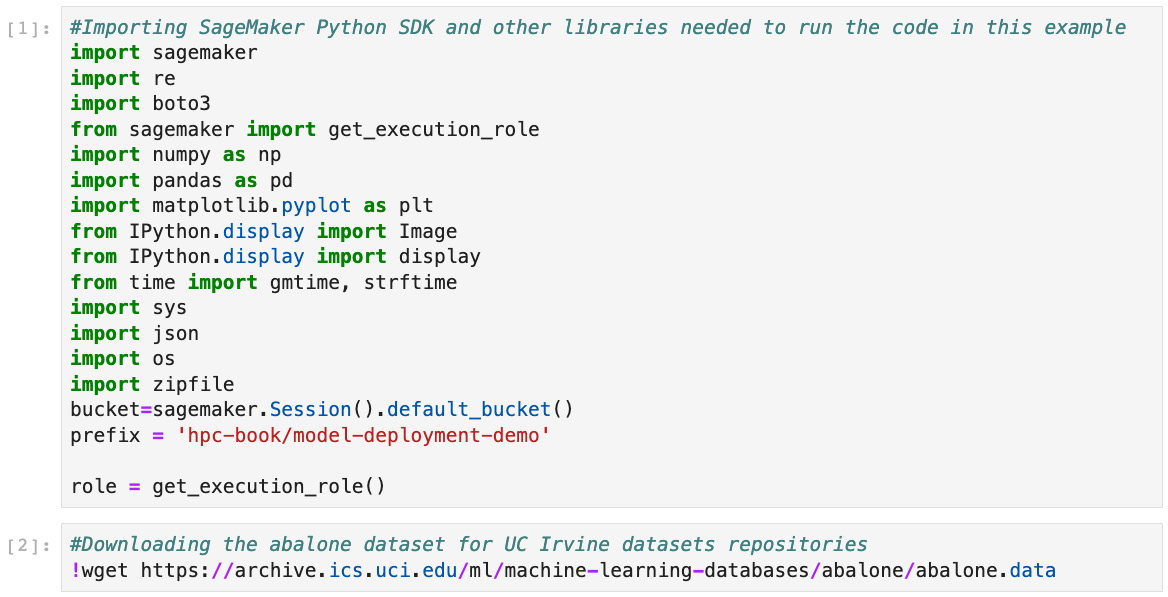
Figure 7.2 – Setting up the packages and bucket in SageMaker and downloading the dataset to be used for model training and inference

2. As shown in Figure 7.3, we can read the data and carry out one hot encoding on the categorical variables.

Figure 7.3 – Doing one hot encoding on categorical variables and displaying the results

3. Figure 7.4 shows the data being split into training, validation, and testing partitions to be used during the model training process.

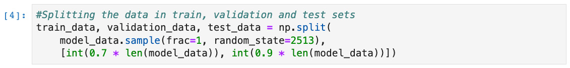
Figure 7.4 – Splitting the data into train, validation, and test sets for model training and testing

4. As shown in Figure 7.5, we can rearrange the columns in the data table in the order that the machine learning model (XGBoost) expects it to be. Furthermore, we can also upload the training and validation data files to an S3 bucket for the model training step.

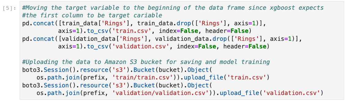
Figure 7.5 – Reorganizing the data and uploading to S3 bucket for training

5. Figure 7.6 shows that we are using SageMaker’s XGBoost container for training our model. It also specifies the data channels for training and validating the model.

Figure 7.6 – Specifying the container for model training along with training and validation data path in S3

As shown in Figure 7.7, we need to define the estimator, the instance type, and instance count, and set various hyperparameters needed by the XGBoost model. We will also start the training job by calling the fit method.

Figure 7.7 – Defining the SageMaker estimator for training and setting up the hyperparameters

Next, let’s create a batch transform job.

Creating a batch transform job for carrying out inference

After creating the transformer object, we need to create a batch transform job. Figure 7.8 shows an example of starting a batch transform job using the transform method call of the batch transformer object. In this transform call, we will specify the location of data in Amazon S3 on which we want to carry out batch inference. In addition, we will also specify the content type of the data (text/csv, in this case), and how the records are split in the data file (each line containing one record, in this case).

Figure 7.8 – Creating a transformer object, preparing data for batch inference, and starting the batch transform job

Figure 7.9 shows an example of reading the results from S3 and then plotting the results (actual versus predictions):

Figure 7.9 – Creating a helper function for reading the results of batch transform, and plotting the results (actual versus predictions)

Figure 7.10 shows the resulting plot:

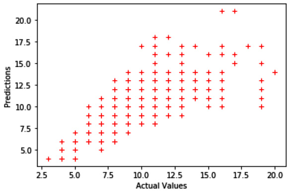
Figure 7.10 – Plot of actual versus prediction Rings values

The code and steps discussed in this section outline the process of training a machine learning model and then carrying out batch inference on the data using the model.

Optimizing a batch transform job

SageMaker Batch Transform also gives us the option of optimizing the transform job using a few hyperparameters, as described here:

• max_concurrent_transforms: The maximum number of HTTP requests that can be made to each batch transform container at any given time. To get the best performance, this value should be equal to the number of compute workers that we are using to run our batch transform job.
• max_payload: This value specifies the maximum size (in MB) of the payload in a single HTTP request sent to the batch transform for inference.
• strategy: This specifies the strategy whether we want to have just one record or multiple records in a batch.

SageMaker Batch Transform is a very useful option to carry out inference on large datasets for use cases that do not require real-time latency and high throughput. The execution of SageMaker Batch Transform can be carried out by using an MLOps workflow, which can be triggered whenever there is new data on which inference needs to be carried out. Automated reports can then be generated using the batch transform job results.

Next, we will learn about deploying a real-time endpoint for making predictions on data using Amazon SageMaker’s real-time inference option.

Real-time inference

As discussed earlier in this chapter, the need for real-time inference arises when we need results with very low latency. Several day-to-day use cases are examples of using real-time inference from machine learning models, such as face detection, fraud detection, defect and anomaly detection, and sentiment analysis in live chats. Real-time inference in Amazon SageMaker can be carried out by deploying our model to the SageMaker hosting services as a real-time endpoint. Figure 7.11 shows a typical SageMaker machine learning workflow of using a real-time endpoint.

Figure 7.11 – Example architecture of a SageMaker real-time endpoint

In this figure, we first read our data from an Amazon S3 bucket. Data preprocessing and feature engineering are carried out on this data using Amazon SageMaker Processing. A machine learning model is then trained on the processed data, followed by results evaluation and post-processing (if any). After that, the model is deployed as a real-time endpoint for carrying out inference on new data in real time with low latency. Also shown in the figure is SageMaker Model Monitor, which is attached to the endpoint in order to detect data and concept drift on new data that is sent to the endpoint for inference. SageMaker also provides the option of registering our machine learning model with the SageMaker Model Registry, for various purposes, such as cataloging, versioning, and automating deployment.

Hosting a machine learning model as a real-time endpoint

Amazon SageMaker provides us with many options to host a model or multiple models as real-time endpoints. We can either use SageMaker Python SDK, the AWS SDK for Python (Boto3), the SageMaker console, or the AWS command-line interface (CLI) to host our models. Furthermore, these endpoints can also host a single model, multiple models in one container in a single endpoint, and multiple models using different containers in a single endpoint. In addition, a single endpoint can also host models containing preprocessing logic as a serial inference pipeline. We will go through these multiple options in the following subsections.

Single model

As mentioned in the preceding section, we can host a model endpoint using multiple options. Here, we will show you how to host an endpoint containing a single model using the Amazon SageMaker SDK. There are two steps involved in creating a single model endpoint using the Amazon SageMaker SDK, as described here:

1. Creating a model object: We need a model object to deploy as an endpoint. The first step to create a real-time endpoint is to use the Model class to create a model object that can be deployed as a HTTPS endpoint. We can also use the model trained in SageMaker. For example, the XGBoost model trained in the example shown in Figure 7.7.
2. Creating the endpoint: The next step is to use the model object’s deploy() method to create an HTTPS endpoint. The deploy method requires the instance type as well as an initial instance count to deploy the model with. This is shown in Figure 7.12:

Figure 7.12 – Calling the deploy method of the XGBoost estimator we trained earlier to deploy our model on a single instance of type ml.m4.xlarge

Figure 7.13 show a custom inference function to serialize the test data, and send it to the real-time endpoint for inference:

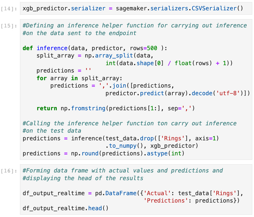
Figure 7.13 – Serializing the data to be sent to the real-time endpoint. Also, creating a helper function to carry out inference using the endpoint

Figure 7.14 displays the inference results for a few records along with the actual values of our target variable—Rings:

Figure 7.14 – Showing a few prediction results versus actual values (Rings)

The endpoint will continue incurring costs as long as it is not deleted. Therefore, we should use real-time endpoints only when we have a use case in which we need inference results in real time. For use cases where we can do inference in batches, we should use SageMaker Batch Transform.

Multiple models

For hosting multiple models in a single endpoint, we can use SageMaker multi-model endpoints. These endpoints can be used to also host multiple variants of the same model. Multi-model endpoints are a very cost-effective method of saving our inference cost for real-time endpoints since the endpoint utilization is generally more when we use multi-model endpoints. We can use business logic to decide on the model to use for inference.

With multi-model endpoints, memory resources across models are also shared. This is very useful when our models are comparable in size and latency. If there are models that have significantly different latency requirements or transactions per second, then single model endpoints for the models are recommended. We can create multi-model endpoints using either the SageMaker console or the AWS SDK for Python (Boto3). We can follow similar steps as those for the creation of a single-model endpoint to create a multi-model endpoint, with a few differences. The steps for Boto3 are as follows:

1. First, we need a container supporting multi-model endpoints deployment.
2. Then, we need to create a model that uses this container using Boto3 SageMaker client.
3. For multi-model endpoints, we also need to create an endpoint configuration, specifying instance types and initial counts.
4. Finally, we need to create the endpoint using the create_endpoint()API call of the Boto3 SageMaker client.

While invoking a multi-model endpoint, we also need to pass a target model parameter to specify the model that we want to use for inference with the data in the request.

Multiple containers

We can also deploy models that use different containers (such as different frameworks) as multi-container endpoints. These containers can be run individually or can also be run in a sequence as an inference pipeline. Multi-container endpoints also help improve endpoint utilization efficiency, hence cutting down on the cost associated with real-time endpoints. Multi-container endpoints can be created using Boto3. The process to create a multi-container endpoint is very similar to creating multi-model and single-model endpoints. First, we need to create a model with multiple containers as a parameter, followed by creating an endpoint configuration, and finally creating the endpoint.

Inference pipelines

We can also host real-time endpoints consisting of two to five containers as an inference pipeline behind a single endpoint. Each of these containers can be a pretrained SageMaker built-in algorithm, our custom algorithm, preprocessing code, predictions, or postprocessing code. All the containers in the inference pipeline function in a sequential manner. The first container processes the initial HTTP request. The response from the first container is sent as a request to the second container, and so on. The response from the final container is sent by SageMaker to the client. An inference pipeline can be considered as a single model that can be hosted behind a single endpoint or can also be used to run batch transform jobs. Since all the containers in an inference pipeline are running on the same EC2 instance, there is very low latency in communication between the containers.

Monitoring deployed models

After deploying a model into production, data scientists and machine learning engineers have to continuously check on the model’s quality. This is because with time, the model’s quality may drift and it may start to predict incorrectly. This may occur because of several reasons, such as a change in one or more variables’ distribution in the dataset, the introduction of bias in the dataset with time, or some other unknown process or parameter being changed.

Traditionally, data scientists often run their analysis every few weeks to check if there has been any change in the data or model quality, and if there is, they go through the entire process of feature engineering, model training, and deployment again. With SageMaker Model Monitor, these steps can be automated. We can set up alarms to detect if there is any drift in data quality, model quality, bias drift in the model and feature distribution drift, and then take corrective actions such as fixing quality issues and retraining models.

Figure 7.15 shows an example of using SageMaker Model Monitor with an endpoint (real-time or asynchronous):

Figure 7.15 – SageMaker Model Monitor workflow for a deployed endpoint (real-time or asynchronous)

First, we need to enable Model Monitor on our endpoint, either at the time of creation or later. In addition, we also need to run a baseline processing job. This processing job analyzes the data and creates statistics and constraints for the baseline data (generally the same dataset with which the model has been trained or validated on). We also need to enable data capture on our SageMaker endpoint to be able to capture the new data along with inference results. Another processing job is then run on fixed intervals to create new statistics and constraints, compares them with the baseline statistics and constraints, and then configures alarms using Amazon CloudWatch metrics in case there is drift in any of the metrics we are analyzing.

In case of a violation in any of the metrics, alarms are generated and these can be sent to a data scientist or machine learning engineer for further analysis and model retraining if needed. Alternatively, we can also use these alarms to trigger a workflow (MLOps) to retrain our machine learning model. Model Monitor is a very valuable tool for data scientists. It can cut down on tedious manual processes for detecting bias and drift in data and model as time progresses after deploying a model.

Asynchronous inference

SageMaker real-time endpoints are suitable for machine learning use cases that have very low latency inference requirements (up to 60 seconds), along with the data size for inference not being large (maximum 6 MB). On the other hand, batch transforms are suitable for offline inference on very large datasets. Asynchronous inference is another relatively new inference option in SageMaker that can process data up to 1 GB and can take up to 15 minutes in processing inference requests. Hence, they are useful for use cases that do not have very low latency inference requirements.

Asynchronous endpoints have several similarities to real-time endpoints. To create asynchronous endpoints, like with real-time endpoints, we need to carry out the following steps:

1. Create a model.
2. Create an endpoint configuration for the asynchronous endpoint. There are some additional parameters for asynchronous endpoints.
3. Create the asynchronous endpoint.

Asynchronous endpoints also have differences when compared to real-time endpoints, as outlined here:

• One main difference from real-time endpoints is that we can scale endpoint instances down to zero when there are no inference requests. This can cut down on the costs associated with having an endpoint for inference.
• Another key difference compared to a real-time endpoint is that instead of passing the payload in line with the request for inference, we upload the data to an Amazon S3 location, and pass on the S3 URI along with the request. Internally, SageMaker keeps a queue of these requests and processes them in the order that they were received. Just like real-time endpoints, we can also do monitoring on the asynchronous endpoint in order to detect model and data drift, as well as new bias.

The code to show a SageMaker asynchronous endpoint is shown in Figure 7.16, using the same model that we created in the batch transform example.

Figure 7.16 – Creating an asynchronous endpoint configuration, followed by the creation of the asynchronous endpoint

Figure 7.17 shows a sample of results for carrying out asynchronous inference on Abalone data used for the batch transform and real-time endpoints examples in previous sections.

Figure 7.17 – Serializing the inference request and calling the asynchronous endpoint to carry out inference on the data.

Figure 7.18 shows the actual and predicted results for a few data points.

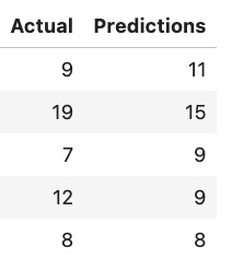
Figure 7.18 – Showing a few predicted results versus the actual values (Rings) using the asynchronous endpoint

In the following section, we will look into the high availability and fault tolerance capabilities of SageMaker endpoints.

The high availability of model endpoints

Amazon SageMaker provides fault tolerance and high availability of the deployed endpoints. In this section, we will discuss various features and options of AWS cloud infrastructure and Amazon SageMaker, that we can use to ensure that our endpoints are fault-tolerant, resilient, and highly available.

Deployment on multiple instances

SageMaker gives us the option of deploying our endpoints on multiple instances. This protects from instance failures. If one instance goes down, then other instances can still serve the inference requests. In addition, if our endpoints are deployed on multiple instances and an availability zone outage occurs or an instance fails, SageMaker automatically tries to distribute our instances across different availability zones, thereby improving the resiliency of our endpoints. It is also a good practice to deploy our endpoints using small instance types spread across different availability zones.

Endpoints autoscaling

Oftentimes, we design our online applications for peak load and traffic. This is also true for machine learning-based applications, where we need hosted endpoints to carry out inference in real time or near real time. In such a scenario, we generally deploy models using the maximum number of instances in order to serve the peak workload and traffic.

If we don’t do this, then our application may start timing out when there are more inference requests than the instances can handle in a combined fashion. This approach results in either the wastage of compute resources or interruptions in the service of our machine learning applications.

To avoid this kind of scenario, Amazon SageMaker lets us configure our endpoints with an autoscaling policy. Using the autoscaling policy, the number of instances on which our endpoint is deployed increases as traffic increases, and decreases as traffic decreases. This helps not only with the high availability of our inference endpoints but also helps in reducing the cost significantly. We can enable autoscaling for a model using either the SageMaker console, the AWS CLI, or the Application Auto Scaling API.

In order to apply autoscaling, we need an autoscaling policy. The autoscaling policy uses Amazon CloudWatch metrics and target values assigned by us to decide when to scale the instances up or down. We also need to define the minimum and maximum number of instances that the endpoint can be deployed on. Other components of the autoscaling policy include the required permissions to carry out autoscaling, a service-linked IAM role, and a cool-down period to wait after a scaling activity before starting the next scaling activity.

Figures 7.19 – 7.22 show autoscaling being configured on an asynchronous endpoint using the Amazon SageMaker console:

1. Figure 7.19 shows that initially the endpoint is just deployed on a single instance:

Figure 7.19 – The endpoint run time settings showing the endpoint being deployed on an instance and autoscaling not being used

After clicking on the Configure auto scaling button, your screen should look like those shown in Figure 7.20 and Figure 7.21.

2. As seen in Figure 7.20, we need to update the minimum and maximum instance counts to 2 and 10, respectively.

Figure 7.20 – Configuring autoscaling on the endpoint to use 2 – 10 instances, depending on traffic (using SageMaker console).

3. As seen in Figure 7.21, we need to update the value for the SageMakerVariantInvocationsPerInstance built-in metric to 200.

Figure 7.21 – Setting the scale in and out time along with the target metric threshold to trigger autoscaling

Once this target value is hit and we are out of the cool-down period, SageMaker will automatically start a new instance or shut down the instance regardless of whether we are above or below the target value.

4. Figure 7.22 shows the results of the endpoint being updated with our autoscaling policy.

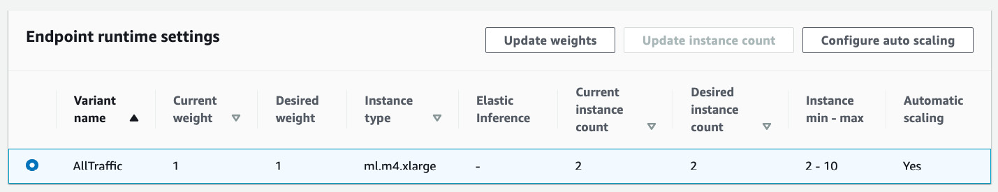
Figure 7.22 – The endpoint running with the autoscaling policy applied

The autoscaling policy can also be updated or deleted after being applied.

Endpoint modification without disruption

We can also modify deployed endpoints without affecting the availability of the models deployed in production. In addition to applying an autoscaling policy as discussed in the previous section, we can also update compute instance configurations of the endpoints. We can also add new model variants and change the traffic patterns between different model variants. All these tasks can be achieved without negatively affecting the endpoints deployed in production.

Now that we’ve discussed how we can ensure that our endpoints are highly available, let’s discuss Blue/green deployments next.

Blue/green deployments

In a production environment where our models are running to make inferences in real time or near real time, it is very important that when we need to update our endpoints that it can happen without any disruption or problems. Amazon SageMaker automatically uses blue/green deployment methodology whenever we update our endpoints. In this kind of scenario, a new fleet, called the green fleet, is provisioned with our updated endpoints. The workload is then shifted from the old fleet, called the blue fleet, to the green fleet. After an evaluation period to make sure that everything is running without any issues, the blue fleet is terminated. SageMaker also provides the following three different traffic-shifted modes for blue/green deployment, allowing us to have more control over the traffic-shifting patterns.

All at once

In this traffic-shifting mode, all of the traffic is shifted at once from the blue fleet to the green fleet. The blue (old) fleet is kept in service for a period of time (called the baking period) to make sure everything is working fine, and performance and functionality are as expected. After the baking period, the blue fleet is terminated all at once. This type of blue/green deployment minimizes the overall update duration, while also minimizing the cost. One disadvantage of the all-at-once method is that regressive updates affect all of the traffic since the entire traffic is shifted to the green fleet at once.

Canary

In canary blue/green deployment, a small portion of the traffic is first shifted from the blue fleet to the green fleet. This portion of the green fleet that starts serving a portion of the traffic is called the canary, and it should be less than 50% of the new fleet’s capacity. If everything works fine during the baking period and no CloudWatch alarms are triggered, the rest of the traffic is also shifted to the green fleet, after which the blue fleet is terminated. If any alarms go off during the baking period, SageMaker rolls back all the traffic to the blue fleet.

An advantage of using canary blue/green deployment is that it confines the blast radius of regressive updates only to the canary fleet and not to the whole fleet, unlike all-at-once blue/green deployment. A disadvantage of using canary deployment is that both the blue and the green fleets are operational for the entire deployment period, thus adding to the cost.

Linear

In linear blue/green deployment, traffic is shifted from the blue fleet to the green fleet in a fixed number of pre-specified steps. In the beginning, the first portion of traffic is shifted to the green fleet, and the same portion of the blue fleet is deactivated. If no alarms go off during the baking period, SageMaker initiates the shifting of the second portion, and so on. If at any point an alarm goes off, SageMaker rolls back all the traffic to the blue fleet. Since traffic is shifted over to the green fleet in several steps, linear blue/green deployment reduces the risk of regressive updates significantly. The cost of the linear deployment method is proportional to the number of steps configured to shift the traffic from the blue fleet to the green fleet.

As discussed in this section, SageMaker has these blue/green deployment methods to make sure that there are safety guardrails when we are updating our endpoints. These blue/green deployment methods ensure that we are able to update our inference endpoints with no or minimal disruption to our deployed machine learning models in a production environment.

Let’s now summarize what we’ve covered in this chapter.

Summary

In this chapter, we discussed the various managed deployment methods available when using Amazon SageMaker. We talked about the suitability of the different deployment/inference methods for different use case types. We showed examples of how we can do batch inference and deploy real-time and asynchronous endpoints. We also discussed how SageMaker can be configured to automatically scale both up and down, and how SageMaker ensures that in case of an outage, our endpoints are deployed to multiple availability zones. We also touched upon the various blue/green deployment methodologies available with Amazon SageMaker, in order to update our endpoints in production.

In a lot of real-world scenarios, we do not have high-performance clusters of instances available for carrying out inference on new and unseen data in real time. For such applications, we need to use edge computing devices. These devices often have limitations on compute power, memory, connectivity, and bandwidth, and need the models to be optimized to be able to use on these edge devices.

In the next chapter, we will extend this discussion to learn about using machine learning models on edge devices.

References

You can refer to the following resources for more information:

• Hosting multiple models on a single endpoint: https://docs.aws.amazon.com/sagemaker/latest/dg/multi-model-endpoints.html
• Amazon EC2 Inf1 instances: https://aws.amazon.com/ec2/instance-types/inf1/
• Using your own inference code with SageMaker Batch Transform: https://docs.aws.amazon.com/sagemaker/latest/dg/your-algorithms-batch-code.html
• Multiple models with different containers behind a single endpoint: https://docs.aws.amazon.com/sagemaker/latest/dg/multi-container-endpoints.html
• Serverless inference on Amazon SageMaker: https://docs.aws.amazon.com/sagemaker/latest/dg/serverless-endpoints.html
• Blue/green deployments using Amazon SageMaker: https://docs.aws.amazon.com/sagemaker/latest/dg/deployment-guardrails-blue-green.html
• Canary traffic shifting: https://docs.aws.amazon.com/sagemaker/latest/dg/deployment-guardrails-blue-green-canary.html
• SageMaker’s Transformer class: https://sagemaker.readthedocs.io/en/stable/api/inference/transformer.html?highlight=transformer
• Amazon SageMaker real-time inference: https://docs.aws.amazon.com/sagemaker/latest/dg/realtime-endpoints-deployment.html
• Best practices for hosting models using Amazon SageMaker: https://docs.aws.amazon.com/sagemaker/latest/dg/deployment-best-practices.html