
Q-learning, as we saw in the previous sections, is quite useful but it does have its drawbacks. For example, as we have to estimate a Q value for each action, there has to be a discrete, limited set of actions. So, what if the action space is continuous or extremely large? Say you are using an RL algorithm to build a portfolio of stocks.
In this case, even if your universe of stocks consisted only of two stocks, say, AMZN and AAPL, there would be a huge amount of ways to balance them: 10% AMZN and 90% AAPL, 11% AMZM and 89% AAPL, and so on. If your universe gets bigger, the amount of ways you can combine stocks explodes.
A workaround to having to select from such an action space is to learn the policy, ![]() , directly. Once you have learned a policy, you can just give it a state, and it will give back a distribution of actions. This means that your actions will also be stochastic. A stochastic policy has advantages, especially in a game theoretic setting.
, directly. Once you have learned a policy, you can just give it a state, and it will give back a distribution of actions. This means that your actions will also be stochastic. A stochastic policy has advantages, especially in a game theoretic setting.
Imagine you are playing rock, paper, scissors and you are following a deterministic policy. If your policy is to pick rock, you will always pick rock, and as soon as your opponent figures out that you are always picking rock, you will always lose. The Nash equilibrium, the solution of a non-cooperative game, for rock, paper, scissors is to pick actions at random. Only a stochastic policy can do that.
To learn a policy, we have to be able to compute a gradient with respect to policy. Contrary to most people's expectations, policies are differentiable. In this section, we will build up a policy gradient step by step and use it to create an advantage actor-critic (A2C) model for continuous control.
The first part in the process of differentiating policies is to look at the advantage we can have by picking a particular action, a, rather than just following the policy, ![]() :
:

The advantage of action a in state s is the value of executing a in s minus the value of s under the policy, ![]() . We measure how good our policy,
. We measure how good our policy, ![]() , is with
, is with  , a function expressing the expected value of the starting state,
 ![]() :
:

Now, to compute the gradient of the policy, we have to do two steps, which are shown inside the expectation in the policy gradient formula:

First, we have to calculate the advantage of a given action, a, with A(s,a). Then we have to calculate the derivative of the weights of the neural network,  , with respect to increasing the probability,
  , that a is picked under policy
 ![]() .
.
For actions with a positive advantage, A(s,a), we follow the gradient that would make a more likely. For actions with a negative advantage, we go in the exact opposite direction. The expectation says that we are doing this for all states and all actions. In practice, we manually multiply the advantage of actions with their increased likelihood gradients.
One thing left for us to look at is how we compute the advantage. The value of taking an action is the reward earned directly as a result of taking the action, as well as the value of the state we find ourselves in after taking that action:

So, we can substitute Q(s,a) in the advantage calculation:

As calculating V turns out to be useful for calculating the policy gradient, researchers have come up with the A2C architecture. A single neural network with two heads that learns both V and ![]() . As it turns out, sharing weights for learning the two functions is useful because it accelerates the training if both heads have to extract features from the environment:
. As it turns out, sharing weights for learning the two functions is useful because it accelerates the training if both heads have to extract features from the environment:

A2C scheme
If you are training an agent that operates on high-dimensional image data, for instance, the value function and the policy head then both need to learn how to interpret the image. Sharing weights would help master the common task. If you are training on lower dimensional data, it might make more sense to not share weights.
If the action space is continuous, ![]() is represented by two outputs, those being the mean,
is represented by two outputs, those being the mean, ![]() , and standard deviation,
, and standard deviation, ![]() . This allows us to sample from a learned distribution just as we did for the autoencoder.
. This allows us to sample from a learned distribution just as we did for the autoencoder.
A common variant of the A2C approach is the asynchronous advantage actor-critic or A3C. A3C works exactly like A2C, except that at training time, multiple agents are simulated in parallel. This means that more independent data can be gathered. Independent data is important as too-correlated examples can make a model overfit to specific situations and forget other situations.
Since both A3C and A2C work by the same principles, and the implementation of parallel gameplay introduces some complexity that obfuscates the actual algorithm, we will just stick with A2C in the following examples.
In this section, we will train an A2C model to swing up and balance a pendulum:

Pendulum gym
The pendulum is controlled by a rotational force that can be applied in either direction. In the preceding diagram, you can see the arrow that shows the force being applied. Control is continuous; the agent can apply more or less force. At the same time, force can be applied in both directions as a positive and negative force.
This relatively simple control task is a useful example of a continuous control that can be easily extended to a stock trading task, which we will look at later. In addition, the task can be visualized so that we can get an intuitive grasp of how the algorithm learns, including any pitfalls.
The pendulum environment is part of the OpenAI Gym, a suite of games made to train reinforcement learning algorithms. You can install it via the command line as follows:
pip install
Before we start, we have to make some imports:
import gym                                           #1

import numpy as np                                   #2

from scipy.stats import norm                         #3
from keras.layers import Dense, Input, Lambda
from keras.models import Model
from keras.optimizers import Adam
from keras import backend as K

from collections import deque                        #4
import random
There are quite a few new imports, so let's walk through them one by one:
- OpenAI's
gymis a toolkit for developing reinforcement learning algorithms. It provides a number of game environments, from classic control tasks, such as a pendulum, to Atari games and robotics simulations. gymis interfaced bynumpyarrays. States, actions, and environments are all presented in anumpy-compatible format.- Our neural network will be relatively small and based around the functional API. Since we once again learn a distribution, we need to make use of SciPy's
normfunction, which helps us take the norm of a vector. - The
dequePython data structure is a highly efficient data structure that conveniently manages a maximum length for us. No more manually removing experiences! We can randomly sample fromdequeusing Python'srandommodule.
Now it is time to build the agent. The following methods all form the A2CAgent class:
def __init__(self, state_size, action_size):

    self.state_size = state_size                       #1
    self.action_size = action_size
    self.value_size = 1

    self.exp_replay = deque(maxlen=2000)               #2


    self.actor_lr = 0.0001                             #3
    self.critic_lr = 0.001
    self.discount_factor = .9


    self.actor, self.critic = self.build_model()       #4

    self.optimize_actor = self.actor_optimizer()       #5
    self.optimize_critic = self.critic_optimizer()
Let's walk through the code step by step:
- First, we need to define some game-related variables. The state space size and the action space size are given by the game. Pendulum states consist of three variables dependent on the angle of the pendulum. A state consists of the sine of theta, the cosine of theta, and the angular velocity. The value of a state is just a single scalar.
- Next, we set up our experience replay buffer, which can save at maximum 2,000 states. Larger RL experiments have much larger replay buffers (often around 5 million experiences), but for this task 2,000 will do.
-
As we are training a neural network, we need to set some hyperparameters. Even if the actor and critic share weights, it turns out that the actor learning rate should usually be lower than the critic learning rate. This is because the policy gradient we train the actor on is more volatile. We also need to set the discount rate,
 . Remember that the discount rate in reinforcement learning is applied differently than it is usually in finance. In finance, we discount by dividing future values by one plus the discount factor. In reinforcement learning, we multiply with the discount rate. Therefore, a higher discount factor,
  , means that future values are less discounted.
- To actually build the model, we define a separate method, which we will discuss next.
- The optimizers for actor and critic are custom optimizers. To define these, we also create a separate function. The optimizers themselves are functions that can be called at training time:
def build_model(self):

    state = Input(batch_shape=(None, self.state_size))          #1

    actor_input = Dense(30,                                     #2
                        activation='relu',
                        kernel_initializer='he_uniform')(state)

    mu_0 = Dense(self.action_size,                              #3
                 activation='tanh',
                 kernel_initializer='he_uniform')(actor_input)

    mu = Lambda(lambda x: x * 2)(mu_0)                          #4

    sigma_0 = Dense(self.action_size,                           #5
                    activation='softplus',
                    kernel_initializer='he_uniform')(actor_input)


    sigma = Lambda(lambda x: x + 0.0001)(sigma_0)               #6

    critic_input = Dense(30,                                    #7
                         activation='relu',
                         kernel_initializer='he_uniform')(state)

    state_value = Dense(1, kernel_initializer='he_uniform')(critic_input)                                                          #8


    actor = Model(inputs=state, outputs=(mu, sigma))            #9
    critic = Model(inputs=state, outputs=state_value)          #10


    actor._make_predict_function()                             #11
    critic._make_predict_function()

    actor.summary()                                            #12
    critic.summary()

    return actor, critic                                       #13
The preceding function sets up the Keras model. It is quite complicated, so let's go through it:
- As we are using the functional API, we have to define an input layer that we can use to feed the state to the actor and critic.
-
The actor has a hidden first layer as an input to the actor value function. It has 30 hidden units and a
reluactivation function. It is initialized by anhe_uniforminitializer. This initializer is only slightly different from the defaultglorot_uniforminitializer. Thehe_uniforminitializer draws from a uniform distribution with the limits , where
  is the input dimension. The default glorot uniform samples from a uniform distribution with the limits , with o being the output dimensionality. The difference between the two is rather small, but as it turns out, the
he_uniforminitializer works better for learning the value function and policy. - The action space of the pendulum ranges from -2 to 2. We use a regular
tanhactivation, which ranges from -1 to 1 first and corrects the scaling later. - To correct the scaling of the action space, we now multiply the outputs of the
tanhfunction by two. Using theLambdalayer, we can define such a function manually in the computational graph. - The standard deviation should not be negative. The
softplusactivation works in principle just likerelu, but with a soft edge:
ReLU versus softplus
- To make sure the standard deviation is not zero, we add a tiny constant to it. Again we use the
Lambdalayer for this task. This also ensures that the gradients get calculated correctly, as the model is aware of the constant added. - The critic also has a hidden layer to calculate its value function.
- The value of a state is just a single scalar that can have any value. The value head thus only has one output and a linear, that is: the default, activation function.
-
We define the actor to map from a state to a policy as expressed by the mean,
 , and standard deviation,
  .
.
- We define the critic to map from a state to a value of that state.
- While it is not strictly required for A2C, if we want to use our agents for an asynchronous, A3C approach, then we need to make the predict function threading safe. Keras loads the model on a GPU the first time you call
predict(). If that happens from multiple threads, things can break._make_predict_function()makes sure the model is already loaded on a GPU or CPU and is ready to predict, even from multiple threads. - For debugging purposes, we print the summaries of our models.
- Finally, we return the models.
Now we have to create the optimizer for the actor. The actor uses a custom optimizer that optimizes it along the policy gradient. Before we define the optimizer; however, we need to look at the last piece of the policy gradient. Remember how the policy gradient was dependent on the gradient of the weights, ![]() , that would make action a more likely? Keras can calculate this derivative for us, but we need to provide Keras with the value of policy
, that would make action a more likely? Keras can calculate this derivative for us, but we need to provide Keras with the value of policy ![]() .
.
To this end, we need to define a probability density function. ![]() is a normal distribution with mean
is a normal distribution with mean ![]() and standard deviation
and standard deviation ![]() , so the probability density function, f, is as follows:
, so the probability density function, f, is as follows:
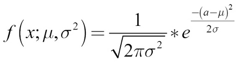
In this term, ![]() stands for the constant, 3.14…, not for the policy. Later, we only need to take the logarithm of this probability density function. Why the logarithm? Because taking the logarithm results in a smoother gradient. Maximizing the log of a probability means maximizing the probability, so we can just use the "log trick," as it is called, to improve learning.
stands for the constant, 3.14…, not for the policy. Later, we only need to take the logarithm of this probability density function. Why the logarithm? Because taking the logarithm results in a smoother gradient. Maximizing the log of a probability means maximizing the probability, so we can just use the "log trick," as it is called, to improve learning.
The value of policy ![]() is the advantage of each action a, times the log probability of this action occurring as expressed by the probability density function, f.
is the advantage of each action a, times the log probability of this action occurring as expressed by the probability density function, f.
The following function optimizes our actor model. Let's go through the optimization procedure:
def actor_optimizer(self):
    action = K.placeholder(shape=(None, 1))                     #1
    advantages = K.placeholder(shape=(None, 1))

    mu, sigma_sq = self.actor.output                            #2

    pdf = 1. / K.sqrt(2. * np.pi * sigma_sq) *
                      K.exp(-K.square(action - mu) / (2. * sigma_sq))                          #3

    log_pdf = K.log(pdf + K.epsilon())                          #4

    exp_v = log_pdf * advantages                                #5

    entropy = K.sum(0.5 * (K.log(2. * np.pi * sigma_sq) + 1.))  #6
    exp_v = K.sum(exp_v + 0.01 * entropy)                       #7
    actor_loss = -exp_v                                         #8

    optimizer = Adam(lr=self.actor_lr)                          #9

    updates = optimizer.get_updates(self.actor.trainable_weights, [], actor_loss)            #10

    train = K.function([self.actor.input, action, advantages], [], updates=updates)                       #11

return train #12- First, we need to set up some placeholders for the action taken and the advantage of that action. We will fill in these placeholders when we call the optimizer.
- We get the outputs of the actor model. These are tensors that we can plug into our optimizer. Optimization of these tensors will be backpropagated and optimizes the whole model.
- Now we set up the probability density function. This step can look a bit intimidating, but if you look closely, it is the same probability density function we defined previously.
- Now we apply the log trick. To ensure that we don't accidentally take the logarithm of zero, we add a tiny constant,
epsilon. - The value of our policy is now the probability of action a times the probability of this action occurring.
- To reward the model for a probabilistic policy, we add an entropy term. The entropy is calculated with the following term:Here, again,

 is a constant 3.14… and
  is the standard deviation. While the proof that this term expresses the entropy of a normal distribution is outside of the scope of this chapter, you can see that the entropy goes up if the standard deviation goes up.
- We add the entropy term to the value of the policy. By using
K.sum(), we sum the value over the batch. - We want to maximize the value of the policy, but by default, Keras performs gradient descent that minimizes losses. An easy trick is to turn the value negative and then minimize the negative value.
- To perform gradient descent, we use the
Adamoptimizer. - We can retrieve an update tensor from the optimizer.
get_updates()takes three arguments,parameters,constraints, andloss. We provide the parameters of the model, that is, its weights. Since we don't have any constraints, we just pass an empty list as a constraint. For a loss, we pass the actor loss. - Armed with the updated tensor, we can now create a function that takes as its input the actor model input, that is, the state, as well as the two placeholders, the action, and the advantages. It returns nothing but the empty list that applies the update tensor to the model involved. This function is callable, as we will see later.
- We return the function. Since we call
actor_optimizer()in theinitfunction of our class, the optimizer function we just created becomesself.optimize_actor.
For the critic, we also need to create a custom optimizer. The loss for the critic is the mean squared error between the predicted value and the reward plus the predicted value of the next state:
def critic_optimizer(self):
    discounted_reward = K.placeholder(shape=(None, 1))          #1

    value = self.critic.output

    loss = K.mean(K.square(discounted_reward - value))          #2

    optimizer = Adam(lr=self.critic_lr)                         #3

    updates = optimizer.get_updates(self.critic.trainable_weights, [], loss)

    train = K.function([self.critic.input, discounted_reward],
                       [],
                       updates=updates)                         #4

    return train
The preceding function optimizes our critic model:
-
Again we set up a placeholder for the variable we need.
discounted_rewardcontains the discounted future value of state as well as the reward immediately earned.
- The critic loss is the mean squared error between the critic's output and the discounted reward. We first obtain the output tensor before calculating the mean squared error between the output and the discounted reward.
- Again we use an
Adamoptimizer from which we obtain an update tensor, just as we did previously. - Again, and finally, as we did previously, we'll roll the update into a single function. This function will become
self.optimize_critic.
For our agent to take actions, we need to define a method that produces actions from a state:
def get_action(self, state):
    state = np.reshape(state, [1, self.state_size])            #1
    mu, sigma_sq = self.actor.predict(state)                   #2
    epsilon = np.random.randn(self.action_size)                #3
    action = mu + np.sqrt(sigma_sq) * epsilon                  #4
    action = np.clip(action, -2, 2)                            #5
    return action
With this function, our actor can now act. Let's go through it:
- First, we reshape the state to make sure it has the shape the model expects.
-
We predict the means and variance,
 , for this action from the model.
- Then, as we did for the autoencoder, we first sample a random normal distribution with a mean of zero and a standard deviation of 1.
- We add the mean and multiply by the standard deviation. Now we have our action, sampled from the policy.
- To make sure we are within the bounds of the action space, we clip the action at -2, 2, so it won't be outside of those boundaries.
At last, we need to train the model. The train_model function will train the model after receiving one new experience:
def train_model(self, state, action, reward, next_state, done):
    self.exp_replay.append((state, action, reward, next_state, done))              #1

     (state, action, reward, next_state, done) = random.sample(self.exp_replay,1)[0]             #2
    target = np.zeros((1, self.value_size))                 #3
    advantages = np.zeros((1, self.action_size))

    value = self.critic.predict(state)[0]                   #4
    next_value = self.critic.predict(next_state)[0]

    if done:                                                #5
        advantages[0] = reward - value
        target[0][0] = reward
    else:
        advantages[0] = reward + self.discount_factor * (next_value) - value
        target[0][0] = reward + self.discount_factor * next_value

    self.optimize_actor([state, action, advantages])        #6
    self.optimize_critic([state, target])
And this is how we optimize both actor and critic:
- First, the new experience is added to the experience replay.
- Then, we immediately sample an experience from the experience replay. This way, we break the correlation between samples the model trains on.
- We set up placeholders for the advantages and targets. We will fill them at step 5.
-
We predict the values for state s and
 .
.
- If the game ended after the current state, s, the advantage is the reward we earned minus the value we assigned to the state, and the target for the value function is just the reward we earned. If the game did not end after this state, the advantage is the reward earned plus the discounted value of the next state minus the value of this state. The target, in that case, is the reward earned plus the discounted value of the next state.
- Knowing the advantage, the action taken, and the value target, we can optimize both the actor and critic with the optimizers we created earlier.
And that is it; our A2CAgent class is done. Now it is time to use it. We define a run_experiment function. This function plays the game for a number of episodes. It is useful to first train a new agent without rendering, because training takes around 600 to 700 games until the agent does well. With your trained agent, you can then watch the gameplay:
def run_experiment(render=False, agent=None, epochs = 3000):
    env = gym.make('Pendulum-v0')                                   #1

    state_size = env.observation_space.shape[0]                     #2
    action_size = env.action_space.shape[0]

    if agent = None:                                                #3
        agent = A2CAgent(state_size, action_size)

    scores = []                                                     #4

    for e in range(epochs):                                         #5
        done = False                                                #6
        score = 0
        state = env.reset()
        state = np.reshape(state, [1, state_size])

        while not done:                                             #7
            if render:                                              #8
                env.render()

            action = agent.get_action(state)                        #9
            next_state, reward, done, info = env.step(action)      #10
            reward /= 10                                           #11
            next_state = np.reshape(next_state, [1, state_size])               #12
            agent.train_model(state, action, reward, next_state, done)                    #13

            score += reward                                        #14
            state = next_state                                     #15

            if done:                                               #16
                scores.append(score)
                print("episode:", e, "  score:", score)

                if np.mean(scores[-min(10, len(scores)):]) > -20:  #17
                    print('Solved Pendulum-v0 after {} iterations'.format(len(scores)))
                    return agent, scores
Our experiment boils down to these functions:
- First, we set up a new
gymenvironment. This environment contains the pendulum game. We can pass actions to it and observe states and rewards. - We obtain the action and state space from the game.
- If no agent was passed to the function, we would create a new one.
- We set up an empty array to keep track of the scores over time.
- Now we play the game for a number of rounds specified by
epochs. - At the beginning of a game, we set the "game over indicator" to
false,scoreto0, and reset the game. By resetting the game, we obtain the initial starting state. - Now we play the game until it is over.
- If you passed
render = Trueto the function, the game would be rendered on screen. Note that this won't work on a remote notebook such as in Kaggle or Jupyter. - We get an action from the agent and act in the environment.
- When acting in the environment, we observe a new state, a reward, and whether the game is over.
gymalso passes an info dictionary, which we can ignore. - The rewards from the game are all negative, with a higher reward closer to zero being better. The rewards can be quite large, though, so we reduce them. Too extreme rewards can lead to too large gradients while training. That would hinder training.
- Before training with the model, we reshape the state, just to be sure.
- Now we train the agent on a new experience. As you have seen, the agent will store the experience in its replay buffer and draw a random old experience to train from.
- We increase the overall reward to track the rewards earned during one game.
- We set the new state to be the current state to prepare for the next frame of the game.
- If the game is over, we track and print out the game score.
- The agent usually does pretty well after 700 epochs. We declare the game solved if the average reward over the last 20 games was better than -20. If that is the case, we will exit the function and return the trained agent together with its scores.
Reinforcement learning algorithms are largely developed in games and simulations where a failing algorithm won't cause any damage. However, once developed, an algorithm can be adapted to other, more serious tasks. To demonstrate this ability, we are now going to create an A2C agent that learns how to balance a portfolio of stocks within a large universe of stocks.
To train a new reinforcement learning algorithm, we first need to create a training environment. In this environment, the agent trades in real-life stock data. The environment can be interfaced just like an OpenAI Gym environment. Following the Gym conventions for interfacing reduces the complexity of development. Given a 100-day look back of the percentile returns of stocks in the universe, the agent has to return an allocation in the form of a 100-dimensional vector.
The allocation vector describes the share of assets the agent wants to allocate on one stock. A negative allocation means the agent is short trading the stock. For simplicity's sake, transaction costs and slippage are not added to the environment. It would not be too difficult to add them, however.
Tip
Tip: The full implementation of the environment and agent can be found at https://www.kaggle.com/jannesklaas/a2c-stock-trading.
The environment looks like this:
class TradeEnv():
    def reset(self):
        self.data = self.gen_universe()                        #1
        self.pos = 0                                           #2
        self.game_length = self.data.shape[0]                  #3
        self.returns = []                                      #4

        return self.data[0,:-1,:]                              #5

    def step(self,allocation):                                 #6
        ret = np.sum(allocation * self.data[self.pos,-1,:])    #7
        self.returns.append(ret)                               #8
        mean = 0                                               #9
        std = 1
        if len(self.returns) >= 20:                            #10
            mean = np.mean(self.returns[-20:])
            std = np.std(self.returns[-20:]) + 0.0001

        sharpe = mean / std                                    #11

        if (self.pos +1) >= self.game_length:                  #12
            return None, sharpe, True, {}
        else:                                                  #13
            self.pos +=1
            return self.data[self.pos,:-1,:], sharpe, False, {}

    def gen_universe(self):                                   #14
        stocks = os.listdir(DATA_PATH)
        stocks = np.random.permutation(stocks)
        frames = []
        idx = 0
        while len(frames) < 100:                              #15
            try:
                stock = stocks[idx]
                frame = pd.read_csv(os.path.join(DATA_PATH,stock),index_col='Date')
                frame = frame.loc['2005-01-01':].Close
                frames.append(frame)
            except:
                e = sys.exc_info()[0]
            idx += 1

        df = pd.concat(frames,axis=1,ignore_index=False)      #16
        df = df.pct_change()
        df = df.fillna(0)
        batch = df.values
        episodes = []                                         #17
        for i in range(batch.shape[0] - 101):
            eps = batch[i:i+101]
            episodes.append(eps)
        data = np.stack(episodes)
        assert len(data.shape) == 3
        assert data.shape[-1] == 100
        return data
Our trade environment is somewhat similar to the pendulum environment. Let's see how we set it up:
- We load data for our universe.
- Since we are stepping through the data where each day is a step, we need to keep track of our position in time.
- We need to know when the game ends, so we need to know how much data we have.
- To keep track of returns over time, we set up an empty array.
- The initial state is the data for the first episode, until the last element, which is the return of the next day for all 100 stocks in the universe.
- At each step, the agent needs to provide an allocation to the environment. The reward the agent receives is the sharpe ratio, the ratio between the mean and standard deviation of returns, over the last 20 days. You could modify the reward function to, for example, include transaction costs or slippage. If you do want to do this, then refer to the section on reward shaping later in this chapter.
- The return on the next day is the last element of the episode data.
- To calculate the Sharpe ratio, we need to keep track of past returns.
- If we do not have 20 returns yet, the mean and standard deviation of returns will be zero and one respectively.
- If we do have enough data, we calculate the mean and standard deviation of the last 20 elements in our return tracker. We add a tiny constant to the standard deviation to avoid division by zero.
- We can now calculate the Sharpe ratio, which will provide the reward for the agent.
- If the game is over, the environment will return no next state, the reward, and an indicator that the game is over, as well as an empty information dictionary in order to stick to the OpenAI Gym convention.
- If the game is not over, the environment will return the next state, a reward, and an indicator that the game is not over, along with an empty information dictionary.
- This function loads the daily returns of a universe of 100 random stocks.
- The selector moves in random order over the files containing stock prices. Some of them are corrupted so that loading them will result in an error. The loader keeps trying until it has 100 pandas DataFrames containing stock prices assembled. Only closing prices starting in 2005 will be considered.
- In the next step, all DataFrames are concatenated. The percentile change in stock price is calculated. All missing values are filled with zero, for no change. Finally, we extract the values from the data as a NumPy array.
- The last thing to do is transform the data into a time series. The first 100 steps are the basis for the agent's decision. The 101st element is the next day's return, on which the agent will be evaluated.
We only have to make minor edits in the A2CAgent agent class. Namely, we only have to modify the model so that it can take in the time series of returns. To this end, we add two LSTM layers, which actor and critic share:
def build_model(self):
	state = Input(batch_shape=(None, #1
			self.state_seq_length,
			self.state_size))
x = LSTM(120,return_sequences=True)(state) #2
x = LSTM(100)(x)
actor_input = Dense(100, activation='relu', #3
		kernel_initializer='he_uniform')(x)
mu = Dense(self.action_size, activation='tanh', #4
		kernel_initializer='he_uniform')(actor_input)
sigma_0 = Dense(self.action_size, activation='softplus',
			kernel_initializer='he_uniform')
			(actor_input)
sigma = Lambda(lambda x: x + 0.0001)(sigma_0)
critic_input = Dense(30, activation='relu',
						kernel_initializer='he_uniform')(x)
state_value = Dense(1, activation='linear',
		kernel_initializer='he_uniform')
		(critic_input)
actor = Model(inputs=state, outputs=(mu, sigma))
critic = Model(inputs=state, outputs=state_value)

actor._make_predict_function()
critic._make_predict_function()

actor.summary()
critic.summary()

return actor, critic
Again, we have built a Keras model in a function. It is only slightly different from the model before. Let's explore it:
- The state now has a time dimension.
- The two
LSTMlayers are shared across actor and critic. - Since the action space is larger; we also have to increase the size of the actor's hidden layer.
- Outputs should lie between -1 and 1, and 100% short and 100% long, so that we can save ourselves the step of multiplying the mean by two.
And that is it! This algorithm can now learn to balance a portfolio just as it could learn to balance before.