Following the long history of modern deep learning being a continuation of quantitative finance with more GPUs, the theoretical foundation of reinforcement learning lies in Markov models.

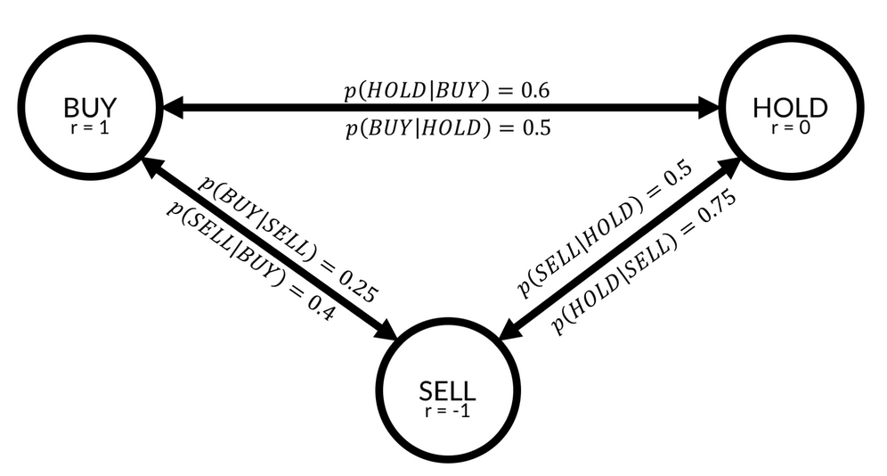
A Markov model describes a stochastic process with different states in which the probability of ending up in a specific state is purely dependent on the state one is currently in. In the following diagram, you can see a simple Markov model describing recommendations given for a stock:

The Markov model

As you can see, there are three states in this model, BUY, HOLD, and SELL. For every two states, there is a transition probability. For example, the probability that a state gets a BUY recommendation if it had a HOLD recommendation in the previous round is described by , which is equal to 0.5. There is a 50% chance that a stock that is currently in HOLD will move to BUY in the next round.

States are associated with rewards. If you own stock, and that stock has a BUY recommendation, the stock will go up, and you will earn a reward of 1. If the stock has a sell recommendation, you will gain a negative reward, or punishment, of -1.

In a Markov model, an agent can follow a policy, usually denoted as . A policy describes the probability of taking action a when in state s. Say you are a trader: you own stock and that stock gets a SELL recommendation. In that case, you might choose to sell the stock in 50% of cases, hold the stock in 30% of cases, and buy more in 20% of cases. In other words, your policy for the state SELL can be described as follows:

Some traders have a better policy and can make more money from a state than others. Therefore, the value of state s depends on the policy, . The value function, V, describes the value of state s when policy is followed. It is the expected return from state s when policy is followed:

The expected return is the reward gained immediately plus the discounted future rewards:

The other value function frequently used in RL is the function Q(s,a), which we have already seen in the previous section. Q describes the expected return of taking action a in state s if policy is followed:

Q and V describe the same thing. If we find ourselves in a certain state, what should we do? V gives recommendations regarding which state we should seek, and Q gives advice on which action we should take. Of course, V implicitly assumes we have to take some action and Q assumes that the result of our actions is landing in some state. In fact, both Q and V are derived from the so-called Bellman equation, which brings us back to the Markov model from the beginning of this section.

If you assume that the environment you operate in can be described as a Markov model, you would really want to know two things. First, you would want to find out the state transition probabilities. If you are in state s, what is the chance ends in state if you take action a? Mathematically, it is as follows:

Equally, you would be interested in the expected reward of being in state s, taking action a and ending up in state :

With this in mind, we can now derive the two Bellman equations for Q and V. First, we rewrite the equation describing V to contain the actual formula for :

We can pull the first reward out of the sum:

The first part of our expectation is the expected reward we directly receive from being in state s and the following policy, :

The preceding equation shows a nested sum. First, we sum over all actions, a, weighted by their probability of occurrence under policy . For each action, we then sum over the distribution of rewards from the transition from state s to the next state, , after action a, weighted by the probability of this transition occurring following the transition probability .

The second part of our expectation can be rewritten as follows:

The expected discounted value of the future rewards after state s is the discounted expected future value of all states, , weighted by their probability of occurrence, , and the probability of action a being taken following policy .

This formula is quite a mouthful, but it gives us a glimpse into the recursive nature of the value function. If we now replace the expectation in our value function, it becomes clearer:

The inner expectation represents the value function for the next step, ! That means we can replace the expectation with the value function, :

Following the same logic, we can derive the Q function as follows:

Congratulations, you have just derived the Bellman equation! For now, pause and take a second to ponder and make sure you really understand the mechanics behind these equations. The core idea is that the value of a state can be expressed as the value of other states. For a long time, the go-to approach to optimizing the Bellman equation was to build a model of the underlying Markov model and its state transition and reward probabilities.

However, the recursive structure calls for a technique called dynamic programming. The idea behind dynamic programming is to solve easier sub-problems. You've already seen this in action in the Catch example. There, we used a neural network to estimate , except for states that ended the game. For these games, finding the reward associated with the state is easy: it is the final reward received at the end of the game. It was these states for which the neural network first developed an accurate estimate of the function Q. From there, it could then go backward and learn the values of states that were further away from the end of the game. There are more possible applications of this dynamic programming and model-free approach to reinforcement learning.

Before we jump into the different kinds of systems that can be built using this theoretical foundation, we will pay a brief visit to the applications of the Bellman equation in economics. Readers who are familiar with the work discussed here will find reference points that they can use to develop a deeper understanding of Bellman equations. Readers unfamiliar with these works will find inspiration for further reading and applications for techniques discussed throughout this chapter.