
We established earlier in this chapter that in order to approximate more complex functions, we need bigger and deeper networks. Creating a deeper network works by stacking layers on top of each other.
In this section, we will build a two-layer neural network like the one seen in the following diagram:

Sketch of a two-layer neural network
The input gets multiplied with the first set of weights, W1, producing an intermediate product, z1. This is then run through an activation function, which will produce the first layer's activations, A1.
These activations then get multiplied with the second layer of weights, W2, producing an intermediate product, z2. This gets run through a second activation function, which produces the output, A2, of our neural network:
z1 = X.dot(W1) + b1

a1 = np.tanh(z1)

z2 = a1.dot(W2) + b2

a2 = sigmoid(z2)
As you can see, the first activation function is not a sigmoid function but is actually a tanh function. Tanh is a popular activation function for hidden layers and works a lot like sigmoid, except that it squishes values in the range between -1 and 1 rather than 0 and 1:

The tanh function
Backpropagation through our deeper network works by the chain rule, too. We go back through the network and multiply the derivatives:
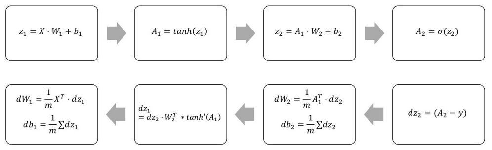
Forward and backward pass through a two-layer neural network
The preceding equations can be expressed as the following Python code:
# Calculate loss derivative with respect to the output
dz2 = bce_derivative(y=y,y_hat=a2)

# Calculate loss derivative with respect to second layer weights
dW2 = (a1.T).dot(dz2)

# Calculate loss derivative with respect to second layer bias
db2 = np.sum(dz2, axis=0, keepdims=True)

# Calculate loss derivative with respect to first layer
dz1 = dz2.dot(W2.T) * tanh_derivative(a1)

# Calculate loss derivative with respect to first layer weights
dW1 = np.dot(X.T, dz1)

# Calculate loss derivative with respect to first layer bias
db1 = np.sum(dz1, axis=0)
Note that while the size of the inputs and outputs are determined by your problem, you can freely choose the size of your hidden layer. The hidden layer is another hyperparameter you can tweak. The bigger the hidden layer size, the more complex the function you can approximate. However, the flip side of this is that the model might overfit. That is, it may develop a complex function that fits the noise but not the true relationship in the data.
Take a look at the following chart. What we see here is the two moons dataset that could be clearly separated, but right now there is a lot of noise, which makes the separation hard to see even for humans. You can find the full code for the two-layer neural network as well as for the generation of these samples in the Chapter 1 GitHub repo:

The two moons dataset
The following diagram shows a visualization of the decision boundary, that is, the line at which the model separates the two classes, using a hidden layer size of 1:

Decision boundary for hidden layer size 1
As you can see, the network does not capture the true relationship of the data. This is because it's too simplistic. In the following diagram, you will see the decision boundary for a network with a hidden layer size of 500:

Decision boundary for hidden layer size 500
This model clearly fits the noise, but not the moons. In this case, the right hidden layer size is about 3.
Finding the right size and the right number of hidden layers is a crucial part of designing effective learning models. Building models with NumPy is a bit clumsy and can be very easy to get wrong. Luckily, there is a much faster and easier tool for building neural networks, called Keras.